Week 2, Lecture 6: Recursive Sequences and Divergence to Infinity
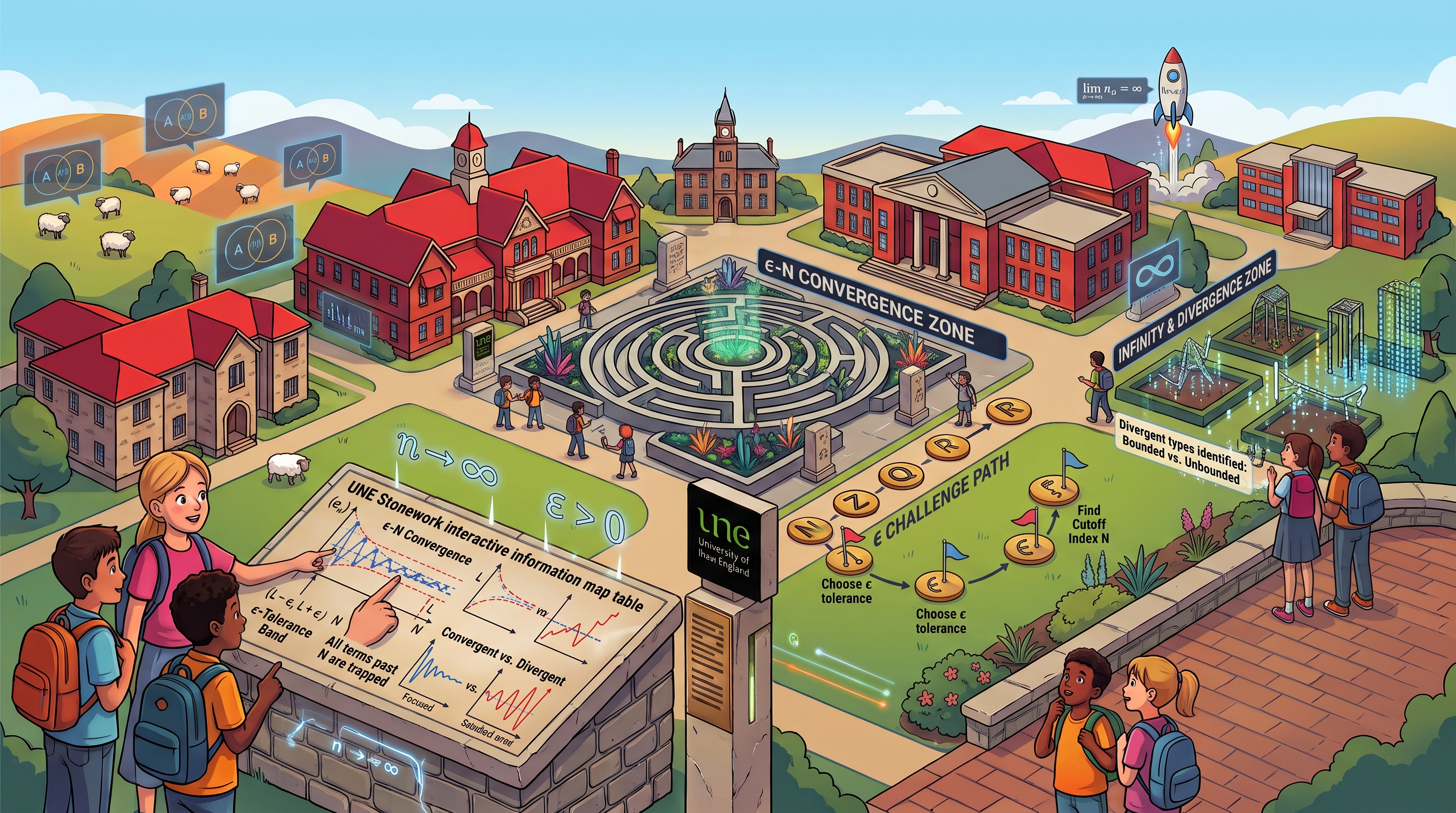
Welcome to Lecture 6: Recursive Sequences and Divergence to Infinity
Take a moment to look back at the conceptual gauntlet you've just run. In the first half of this week, you built the rigorous $\epsilon\text{-}N$ foundation of limits. In Lecture 5, you learned how to trap complex, unpredictable sequences using physical boundaries like the Monotone Convergence and Squeeze theorems. You have successfully dismantled the "magic" of calculus and replaced it with unbreakable mathematical logic.
Today, as we close out Week 2, we are tying up two crucial loose ends. First, we will take a deeper dive into Recursive Sequences. You saw a brief, successful glimpse of these when we used the MCT, but today we will fully unpack how to analyze sequences that don't give you a clear map, but instead dynamically generate themselves one step at a time based on their own history. Second, we will look at the ultimate rebellious sequences: those that shatter their ceilings and exhibit Divergence to Infinity.
Up until now, our working definition of divergence has just been a negative statement: "it fails to converge." But a sequence that bounces chaotically between $-1$ and $1$ is physically very different from a sequence rocketing upward forever. Today, we will build a formal, rigorous definition for infinity itself. Mastering this precise language of recursion and unbounded growth is the essential bridge to our next major chapter—Infinite Series—where we will need to understand exactly how mathematical structures accumulate, and exactly what happens when they explode. Let's finish the week strong!
📌 Lecture 6 Topics
How Recursive Sequences Trap Infinity
You have made it to the final hurdle of sequence limits! In this episode, we tackle the most unruly mathematical behaviors: sequences that build themselves step-by-step and sequences that shatter all ceilings. Join us as we explore how to calculate the impossible using recursive error contraction, reveal the "cheat code" for the 4-Step MCT strategy, and trade our microscopic epsilon for a massive threshold $M$. Finally, we put geometric and linear growth in a mathematical drag race to prove exactly why exponential scaling leaves linear equations in the dust.
1. What is a Recursive Sequence?
Up until now, almost every sequence you have worked with has been explicit. An explicit sequence gives you a direct mathematical formula (like $a_n = \frac{1}{n}$). If you want to know the 100th term, you just plug in $n=100$ and teleport straight to the answer.
A recursive sequence operates entirely differently. Instead of a direct map, it gives you a starting position (like $a_1 = 2$) and a rule for how to take the next step based on where you currently stand. Mathematically, this rule is written as $a_{n+1} = f(a_n)$. The sequence uses its own past to generate its future. If you want to calculate the 100th term, you cannot teleport; you must know the 99th term first.
Existence Before Algebra (The Limit Prerequisite)
When you are handed a recursive formula like $a_{n+1} = f(a_n)$ and asked to find its limit, your mathematical reflexes should immediately kick in. Your natural instinct is likely to apply the Algebraic Limit Laws: if the sequence converges to some final destination $L$, then as $n$ goes to infinity, both the "current step" ($a_n$) and the "next step" ($a_{n+1}$) must eventually become $L$. You can simply write $L = f(L)$ and solve for $L$ using basic algebra.
This algebraic instinct is absolutely correct and highly powerful. It is exactly how professional mathematicians solve these problems. However, this algebraic tool has a strict built-in safety switch: the equation $L = f(L)$ is only legally and mathematically valid after you have proven that a finite limit $L$ actually exists.
⚠️ The Fibonacci Boundary Check
To see why this existence prerequisite is so important, consider the famous Fibonacci sequence: $f_0 = 1, f_1 = 1$, and $f_{n+2} = f_{n+1} + f_n$ ($1, 1, 2, 3, 5, 8, \dots$). We intuitively know this sequence grows forever to infinity.
But what if we skip the boundary check? Skipping the check means we don't bother to mathematically prove the sequence is trapped by a ceiling. Instead, we just blindly assume it eventually flattens out at some finite limit $L$.
If it flattens out at $L$, then eventually every term in the formula ($f_{n+2}$, $f_{n+1}$, and $f_n$) just becomes $L$. Look what happens when we plug that assumption into the Fibonacci rule:
Subtracting $L$ from both sides leaves us with exactly $L = 0$.
The algebra worked flawlessly and output $0$. But this completely contradicts reality—the sequence is rocketing away from zero!
The Takeaway: Algebra is like a blind machine. If you feed it an equation and ask "where does this stop?", it will confidently crunch the numbers and hand you an answer, even if the sequence is actually rocketing off into outer space. You must use boundary theorems (like the Monotone Convergence Theorem) first to guarantee a limit actually exists before your algebraic tools can be trusted.
2. Approximating the Impossible: Calculating $\sqrt{2}$
Why should we care about recursive sequences? Because they allow us to calculate the impossible.
Imagine you are an ancient mathematician trying to calculate the diagonal of a $1 \times 1$ square. The answer is $\sqrt{2}$. But $\sqrt{2}$ is an irrational number—it is an infinite, non-repeating decimal. You cannot write it as a simple fraction, and you certainly don't have a calculator. How do you find its value using only basic arithmetic?
The answer is to build a recursive machine. You design a formula where you plug in a bad guess, and the formula spits out a slightly better fraction. You take that new fraction, plug it back into the formula, and get an even better one.
💡 Demystifying the Magic: Where does the formula come from?
Math textbooks love to drop formulas from the sky. Let's look at exactly how we invent a recursive machine to find $\sqrt{2}$. We start with the basic equation and use an algebraic trick to turn it into a loop:
Add $x$ to both sides so we have $x$ in multiple places:
Factor out the $x$ on the left:
Divide by $(x + 1)$ to isolate $x$:
The Machine is Built! We just replace the $x$ on the left with our "next step" ($a_{n+1}$) and the $x$'s on the right with our "current step" ($a_n$). We now have a recursive formula that zeroes in on $\sqrt{2}$!
Let's test our new machine. We will start with a terrible guess ($a_0 = 1$) and see what fractions it generates:
Notice how the numbers bounce above and below the true value of $\sqrt{2}$ ($\approx 1.4142$), but the bounces are getting smaller. This brings us to a powerful proof strategy.
What is "Error Contraction"?
When a sequence bounces up and down, we cannot use the Monotone Convergence Theorem (because it isn't moving in just one direction).
Instead, we use a strategy called Error Contraction. Instead of looking at the sequence numbers themselves, we look at the gap between our sequence and the target. This gap is our "Error."
The Concept: If you are guessing a number, and with every single guess, the size of your error gets chopped in half, what eventually happens? The error shrinks to zero. If the error reaches zero, you have hit the exact target.
🎯 Rigorous Proof of Convergence via Error Contraction
Let's define our Error at step $n$ (the absolute distance to the target) as $\text{Error}_n = |a_n - \sqrt{2}|$.
We want to prove that taking a step in our recursive machine forces this error to shrink significantly.
Step 1: Calculate the Error for the next step ($n+1$)
Step 2: Find a common denominator to combine the terms
Step 3: Factor out the previous Error ($|a_n - \sqrt{2}|$)
(By factoring out $(1 - \sqrt{2})$ from the numerator, we can separate our previous error from the rest of the garbage)
(If the algebra in the numerator seems to jump too fast, here is the exact breakdown of how we separate the previous error from the rest of the terms)
- Group the terms: Rearrange the numerator to group the $a_n$ terms together and the constants together: $a_n - \sqrt{2}a_n + 2 - \sqrt{2}$.
- Factor the groups: Pull $a_n$ out of the first pair, and pull $\sqrt{2}$ out of the second pair (remembering that $2 = \sqrt{2} \cdot \sqrt{2}$):
$$a_n(1 - \sqrt{2}) + \sqrt{2}(\sqrt{2} - 1)$$
- Match the factors: To make the pieces in the parentheses match, rewrite $\sqrt{2}(\sqrt{2} - 1)$ as $-\sqrt{2}(1 - \sqrt{2})$. Now factor $(1 - \sqrt{2})$ out of the entire numerator:
$$(1 - \sqrt{2})(a_n - \sqrt{2})$$
- Separate the absolute values: The absolute value of a product is the product of the absolute values. Since $|1 - \sqrt{2}| = \sqrt{2} - 1$ and $|a_n + 1| = a_n + 1$, we are left with:
Step 4: Prove the Shrinkage
We now have this relationship: $\text{Error}_{n+1} = \left(\frac{\sqrt{2} - 1}{a_n + 1}\right) \cdot \text{Error}_n$.
Look at the fraction multiplying our old error. We know $\sqrt{2} - 1 \approx 0.414$. We also know our sequence terms $a_n$ are always at least $1$, making the denominator $(a_n + 1)$ at least $2$.
Therefore, the fraction $\frac{0.414}{\text{at least } 2}$ is safely smaller than $\frac{1}{2}$. We have successfully proven that our error gets chopped by more than half every single step:
Because multiplying by a fraction less than $1$ repeatedly drives a number to zero (e.g., $\left(\frac{1}{2}\right)^n \to 0$), the Squeeze Theorem forces our Error sequence to exactly $0$. The sequence has no choice but to converge exactly to $\sqrt{2}$. $\blacksquare$
3. The 4-Step Strategy for Recurrences
🛠️ The 4-Step Strategy
- Step 1: Prove Boundedness. Use mathematical induction to show the sequence is trapped by a ceiling ($a_n \le M$) or a floor ($a_n \ge m$).
- Step 2: Prove Monotonicity. Use induction again to show the sequence only moves in one direction: $a_{n+1} > a_n$ (increasing) or $a_{n+1} < a_n$ (decreasing).
- Step 3: Invoke the MCT. Now that you have proven the sequence is physically trapped and moving in one direction, the Monotone Convergence Theorem guarantees a finite limit $L$ exists.
- Step 4: Solve Algebraically. Because you legally proved $L$ exists in Step 3, you can now safely take the limit of both sides of the formula ($a_{n+1} = f(a_n)$) to find exactly what $L$ is.
💡 The "Cheat Code" for Step 1
How do you know what number to use for your boundary in Step 1? You cheat. Do Step 4 on a piece of scratch paper first. If your algebraic scratch-work tells you the limit is going to be 2, then you immediately know that 2 is the perfect ceiling to use for your boundedness proof.
🎯 Worked Example: The Nested Radical
Let's define a sequence by $x_1 = \sqrt{2}$, and $x_{n+1} = \sqrt{2 + x_n}$. What is its limit?
(Scratchpad math: If we assume a limit $L$ exists, $L = \sqrt{2+L}$, which squares to $L^2 - L - 2 = 0$. Factoring gives $(L-2)(L+1)=0$. Since our terms are positive, the limit must be 2. Now we know 2 is the ceiling we need to prove!)
Step 1: Prove Boundedness (Show it never passes 2)
- Base Case: For $n=1$, $x_1 = \sqrt{2} \approx 1.414$, which is strictly less than $2$.
- Inductive Assumption: Assume that for some step $k$, $x_k < 2$.
- Inductive Step: We must prove $x_{k+1} < 2$.
$$x_{k+1} = \sqrt{2 + x_k}$$Because we assumed $x_k < 2$, we can replace $x_k$ with 2 to create a strict inequality:$$x_{k+1} < \sqrt{2 + 2} = \sqrt{4} = 2$$By induction, the sequence is bounded above by 2 forever.
Step 2: Prove Monotonicity (Show it is always increasing)
- Base Case: $x_2 = \sqrt{2 + \sqrt{2}} \approx 1.84$. This is greater than $x_1$ ($1.414$). So, $x_2 > x_1$.
- Inductive Assumption: Assume that at step $k$, the sequence increased: $x_{k} > x_{k-1}$.
- Inductive Step: We must prove it increases at the next step: $x_{k+1} > x_k$.
$$x_{k+1} = \sqrt{2 + x_k}$$Because we assumed $x_k > x_{k-1}$, we can swap them out to maintain the inequality:$$x_{k+1} > \sqrt{2 + x_{k-1}}$$But notice that $\sqrt{2 + x_{k-1}}$ is exactly the definition of $x_k$. Therefore, $x_{k+1} > x_k$. By induction, it is strictly increasing.
Step 3: Invoke the MCT
Because the sequence is strictly increasing (Step 2) and securely trapped below a ceiling of 2 (Step 1), the Monotone Convergence Theorem formally guarantees that a finite limit $\lim x_n = L$ exists.
Step 4: Solve Algebraically
Because Step 3 gave us mathematical permission, we can now take the limit of the formula $x_{n+1} = \sqrt{2 + x_n}$. Every term becomes $L$:
Factoring gives $(L-2)(L+1) = 0$. Since our sequence consists entirely of positive square roots, the limit cannot be $-1$. The limit is exactly $2$. $\blacksquare$
4. Infinity as a Limit ($M\text{-}N$ Definition)
Earlier this week, you mastered the $\epsilon\text{-}N$ definition of a limit. In that definition, $\epsilon$ represented a tiny, microscopic boundary used to trap a sequence that was settling down to a single finite number.
But how do we rigorously describe a sequence that never settles down, but instead rockets upward forever? A tiny boundary $\epsilon$ is absolutely useless here. Instead, we need to prove that the sequence can break through any ceiling we put in its way. We replace the tiny error $\epsilon$ with a massive threshold $M$.
A sequence tends to positive infinity ($\lim_{n\to\infty} a_n = \infty$) if for every massive threshold $M$, there is a specific step $N$ in the sequence where all terms after that step permanently cross the threshold:
Similarly, $\lim_{n\to\infty} a_n = -\infty$ if for every deep floor $M < 0$, there exists an $N \in \mathbb{N}$ such that $n > N \implies a_n < M$.
VISUALIZATION: The $M\text{-}N$ Threshold Test for $\lim_{n\to\infty} \sqrt{n} = \infty$
🎯 Worked Example: Proving $\lim_{n\to\infty} \sqrt{n} = \infty$
Just like the $\epsilon\text{-}N$ proofs from earlier, $M\text{-}N$ proofs follow a predictable game: the challenger hands you an arbitrary threshold $M$, and you must use algebra to find the exact step $N$ where the sequence permanently breaks past it.
Step 1: The Challenge
Let $M > 0$ be an arbitrary, massively large threshold given to us.
Step 2: The Algebraic Scratch-Work
We want our sequence to break the threshold. So, we set up the inequality $a_n > M$ and solve for $n$:
Step 3: The Formal Choice
Based on our scratch-work, we choose our cutoff index $N$ to be any natural number greater than $M^2$.
Step 4: The Proof
If we take any step $n > N$, it immediately follows that $n > M^2$. Taking the square root of both sides of that inequality, we get exactly what we needed to show:
Because we proved the sequence eventually exceeds any arbitrary threshold $M$, we have formally proven that $\lim_{n\to\infty} \sqrt{n} = \infty$. $\blacksquare$
5. Growth Rates: Geometric vs. Linear Divergence
In Section 4, we built the $M\text{-}N$ test to formally prove if a sequence diverges to infinity. But in applied mathematics, just knowing a sequence explodes is rarely enough—we usually need to know how fast it explodes.
The Two Flavors of Infinity
Consider two different sequences that both diverge to infinity:
- Linear Divergence ($b_n = \alpha n + \beta$): This is steady, additive growth. If you have a sequence like $b_n = 5n + 1000$, you are just adding 5 at every single step. It marches to infinity at a constant, predictable speed, much like walking up a staircase.
- Geometric Divergence ($a_n = c r^n$): This is multiplicative, compounding growth. If you have a sequence like $a_n = 2^n$ (with a ratio $r > 1$), you are multiplying the previous term by 2 at every step. The growth accelerates violently as the numbers get larger.
Understanding the difference between these two growth rates becomes critically important in computer science when analyzing how fast an algorithm works. If the time it takes a program to run grows linearly as you give it more data, the algorithm scales well. But if the time grows geometrically, the algorithm will quickly exceed all available computational resources.
We need a rigorous mathematical way to prove that geometric growth is truly in a different weight class than linear growth. To do this, we put them in a race by looking at their ratio: $\frac{a_n}{b_n}$. If this ratio tends to $\infty$, the sequence on top is the undisputed winner.
💡 The Algebraic Trick: Cracking Open $r^n$
To prove this, we need to compare an exponential term ($r^n$) directly to a linear term ($n$). How do we get the $n$ out of the exponent so we can do algebra with it?
The Trick: Because our geometric ratio $r$ is strictly greater than 1, we can split it into exactly $1$ plus some positive remainder $\epsilon$. So, $r = 1 + \epsilon$. Once we do this, we can use the Binomial Formula to expand $(1 + \epsilon)^n$ and expose the standard polynomials hiding inside it.
🎯 Theorem: Geometric Sequences Diverge Faster Than Linear Ones
Let $a_n = c r^n$ be a geometric sequence with $r > 1$ and $c > 0$. Let $b_n = \alpha n + \beta$ be a linear sequence ($\alpha > 0$). We will prove that $\frac{a_n}{b_n} \to \infty$ by focusing on the core engine of the sequences: we will prove $\frac{r^n}{n} \to \infty$.
Step 1: The Binomial Expansion
Write $r = 1 + \epsilon$ for some $\epsilon > 0$. By the Binomial Formula, expanding $(1 + \epsilon)^n$ gives us a sum of positive terms:
Because every term is positive, if we chop off everything after the first three terms, the right side becomes strictly smaller. This gives us a guaranteed floor:
Step 2: Divide by the Linear Engine ($n$)
Our goal is to analyze the ratio $\frac{r^n}{n}$, so let's divide our entire inequality by $n$:
Step 3: Evaluate the Limit
Let's look at what happens to the right side of our inequality as $n \to \infty$:
- The $\frac{1}{n}$ term shrinks to $0$.
- The $\epsilon$ term is just a constant.
- The $\frac{n-1}{2}\epsilon^2$ term has an $n$ in the numerator, meaning it grows without bound (to $\infty$).
Because the right side of our inequality explodes to infinity, the left side ($\frac{r^n}{n}$) is physically pushed to infinity as well. Because the geometric sequence contains an $n^2$ engine hidden inside its expansion, it completely overpowers and dominates any linear polynomial. $\blacksquare$
The Mechanics of the Infinite
Before we officially close out Week 2, let's consolidate the exact mathematical machinery you just built. You didn't just read definitions today; you forged four distinct analytical tools to handle the most unpredictable sequences in calculus:
You learned how to mathematically trap recursive sequences. By proving boundedness and monotonicity via induction, you earn the legal right to extract the limit algebraically.
For sequences that oscillate as they converge (like our $\sqrt{2}$ approximation), you learned to analyze the distance to the target, proving that the gap shrinks by a strict fraction at every single step.
You replaced the tiny $\epsilon$ corridor with a massive threshold $M$. Proving divergence to infinity simply means calculating the cutoff $N$ where the sequence permanently breaches any ceiling.
You raced divergent sequences against each other. Using the Binomial Formula, you rigorously proved that geometric compounding ($r^n$) always mathematically overpowers linear growth ($n$).
🏁 You Have Mastered the Infinite
Take a massive, well-deserved breath and appreciate what you have just accomplished. You have officially crossed one of the most challenging and rewarding milestones in this entire course! You didn't just crunch numbers today—you learned how to tame mathematical chaos.
Taming Recurrences
You built a recursive machine to calculate the impossible (like $\sqrt{2}$) and locked down unpredictable, self-referencing sequences using the rigorous 4-Step MCT Strategy.
The $M\text{-}N$ Threshold
You proved exactly what it means to rocket upward forever. By replacing the tiny $\epsilon$ boundary with a massive threshold $M$, you captured and defined divergence to infinity.
Growth Rate Races
You raced infinite growths against each other, proving rigorously why geometric sequences easily overpower linear ones, and why algorithms fail when pushed too far.
The Grand Scheme: Why Did We Do This?
Why did we push so hard today to lock down these behaviors? Because everything you just conquered is the exact engine we need for our next major topic: Functions. When we transition from isolated, discrete sequence steps into a world of fluid, continuous curves, we will be relying entirely on the rigorous boundary checks and error mechanics you just mastered today to evaluate limits of functions.
Looking Ahead to Week 3: Functions and Continuity
Next week, we move off the discrete stepping stones of sequences and into the continuous world of mapping inputs to outputs.
- We will explore Transcendental Functions like logarithms and exponentials.
- We will take the distance boundaries we used today and use them to formally define exactly what it means for a curve to be continuous without any breaks or gaps.
- We will map domain restrictions, inverse functions, and bijective mappings.
You are officially thinking like a true mathematician. You now have the exact boundary and limit mechanics needed to tackle continuous space.
Be proud of this win, let the algebra settle, and I will see you in the next module!
Ready to test your understanding?
Work through the progressive interactive problems to lock in these foundational concepts.
Launch Interactive Problem Stepper ➔