Week 3, Lecture 7: Functions, Domains, and Inverses

Welcome to Lecture 7: Mapping the Continuum
If the rigorous logic and $\epsilon$-$N$ proofs of Weeks 1 and 2 felt demanding, take a deep breath. You have already done the hardest part: building the logical machinery required for real analysis. Over the past two weeks, we focused entirely on sequences—lists of distinct, isolated numbers acting like stepping stones across a river.
Now, we are going to connect those dots. In Week 3, we transition from the discrete stepping stones of sequences into the continuous, fluid world of functions. This shift is crucial. The ultimate goal of this course is to prepare you for calculus—the mathematics of continuous change, like tracing the real-time velocity of an object, the smooth growth of a curve, or the volume of a solid. To analyze how a curve changes and moves, we must first rigorously define the underlying rules that govern the curve itself.
We aren't introducing entirely new math today; rather, we are putting a formal analytical lens on algebra you likely already know. We will view a function not just as a formula to be calculated, but as a rigid structural mapping that assigns every element in a domain to exactly one element in a codomain. Today, we will solidify these mappings, explore the exact geometric and algebraic conditions required to run a function in reverse (invertibility), and lock in the foundational algebraic curves (linear, power, and rational functions) that we will be bending and stretching throughout the rest of the term.
The Factory Floor: Logic Machines, Safety Limits, and Reversing the Irreversible
Explore the mathematics factory floor. We translate abstract function notation into physical machines, establish the safety manual of domain constraints, and unpack why reverse-engineering a parabola requires a mathematical scalpel.
1. The Natural Domain, Codomain, and Range
In set theory and real analysis, a function $f: X \to Y$ is a strict structural mapping. It assigns every single element from a starting set $X$, which is called the domain, to exactly one element in a destination set $Y$, which is called the codomain.
🔍 The Target vs. The Hits (Codomain vs. Range)
It is a common mistake to confuse the codomain with the range. They are distinct concepts in pure mathematics:
- The Codomain ($Y$): The entire set of possible outputs where the function's results are allowed to land. For most functions in this unit, the codomain is simply the set of all real numbers, $\mathbb{R}$.
- The Range ($R$): The specific subset of the codomain consisting of elements that are actually hit by the function, meaning they are actual values of $f$ for some arguments. For example, the function $f(x) = x^2$ mapping $\mathbb{R} \to \mathbb{R}$ has a codomain of all real numbers, but its range is strictly $[0, \infty)$ because a square cannot be negative.
When a function is given to us strictly as an algebraic formula without an explicit domain, that formula may make perfect sense for some inputs but completely break down for others. We must determine the mathematical boundaries ourselves.
Definition: The Natural Domain
The natural domain of a function $f(x)$ is the largest possible subset of the real numbers $\mathbb{R}$ where the formula is well-defined and mathematically valid.
📐 Notation Refresher: Intervals on the Real Line
Classification of Mappings: Injective, Surjective, and Bijective
Not all functions behave the same way when dropping inputs into the codomain. We classify functions based on two critical questions: Do any inputs collide into the same output? and Are any potential outputs left empty?
1. Injective (One-to-One)
No Collisions
Every input maps to a unique output. Misses are allowed (the codomain isn't fully covered), but no two inputs ever share a destination.
2. Surjective (Onto)
No Misses
Every element in the codomain is hit by at least one input. Collisions are allowed, but the Range is exactly equal to the Codomain.
3. Bijective
Perfect Pairing
The function is both injective and surjective. Every input has exactly one output, and every output has exactly one input.
Why this matters for Calculus: Only a perfect bijection can be safely run in reverse. If a function has collisions (not injective), reversing it would mean one output points back to multiple inputs—creating a paradox. If a function has misses (not surjective), reversing it would cause the reverse function to hit undefined empty space.
To truly understand how functions behave geometrically, we must look beyond algebraic formulas and examine their graphs. In formal set theory, a function is not merely a dynamic rule; it is defined statically by its graph.
Definition: The Graph of a Function
Let $f: X \to Y$ be a function. The graph of $f$ is the subset of the Cartesian product $X \times Y$ defined by the set of all coordinate pairs: $$\text{Graph}(f) = \{ (x, f(x)) \mid x \in X \}$$
This formal definition reveals a powerful visual test. A subset of the Cartesian plane $X \times Y$ represents a valid function if and only if every vertical line $x = c$ intersects the graph in at most one point. Why? Because a single input $x$ cannot map to multiple outputs without violating the core definition of a function.
The Geometry of Inverse Graphs
When a function $f: X \to Y$ is bijective (both injective and surjective), it possesses an inverse function $g: Y \to X$ (commonly denoted $f^{-1}$). What is the relationship between the graph of $f$ and the graph of its inverse?
If the point $(a, b)$ lies on the graph of $f$, meaning $f(a) = b$, then by definition of the inverse, $f^{-1}(b) = a$, meaning the point $(b, a)$ must lie on the graph of $f^{-1}$. Geometrically, switching the coordinates from $(a, b)$ to $(b, a)$ corresponds to a mirror reflection across the diagonal line $y = x$.
🪞 The Horizontal Line Test and Invertibility
Because the graph of the inverse is a reflection across $y = x$, we can determine if a function is invertible just by looking at its graph:
- Vertical Line Test: Determines if a curve is a valid function (each input has only one output).
- Horizontal Line Test: Determines if a function is injective (each output comes from only one input). If any horizontal line intersects the graph more than once, the function fails the test, and no standard inverse can exist unless we restrict its domain.
🏛️ Historical Aside: From Leibniz to Dirichlet — The Evolution of the Function Concept
The modern concept of a function did not appear overnight. It evolved over centuries through a dramatic shift—moving away from rigid algebraic formulas and curve-fitting toward abstract sets, domains, and rules of correspondence.

1. Leibniz and the Birth of the Term (1692)
The story begins with Gottfried Wilhelm Leibniz, who first used the Latin term functio to describe quantities related to geometric curves, such as tangents or coordinates. Shortly after, his collaborator Johann Bernoulli published the first formal definition: “a quantity composed in any manner whatsoever from a variable magnitude and constants.” To them, a function was strictly tied to a formula.

Johann Bernoulli's Analytical View
Johann Bernoulli championed the idea that functions were expressions built out of algebra. If an expression couldn't be written out as a clear analytical formula, it fell outside standard mathematical analysis.

2. Euler and the Reign of the Formula (1748)
Johann Bernoulli's brilliant student, Leonhard Euler, cemented the formula-based view in his landmark work Introductio in analysin infinitorum. Euler also popularized the notation f(x). For Euler, functions were powerful analytical expressions; anything requiring discontinuous rules or broken graphs was treated as a bizarre exception.
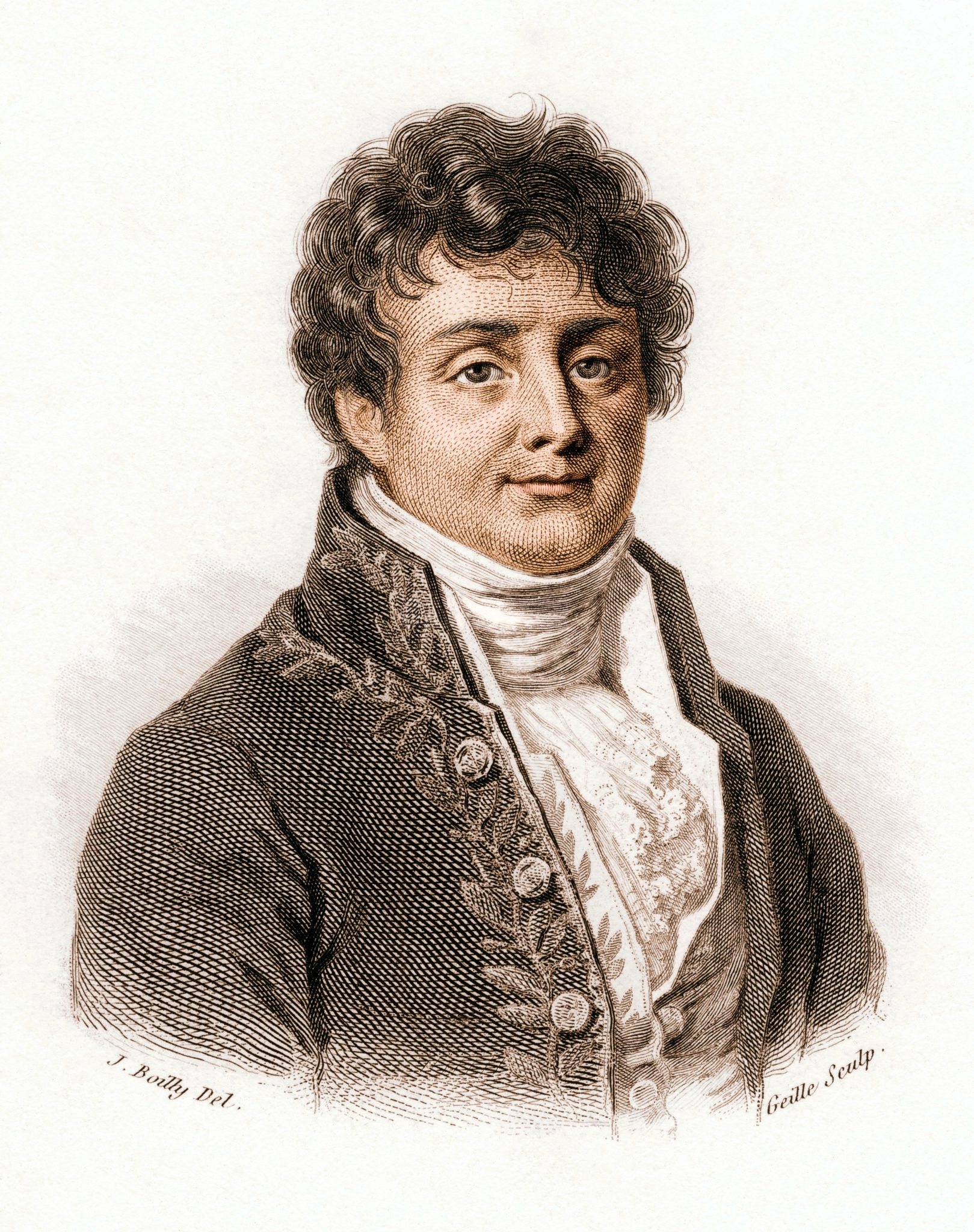
3. The Fourier Shockwave (Early 19th Century)
The neat world of formula-bound functions broke down when Joseph Fourier showed that arbitrary, jagged curves could be expressed using infinite sums of sines and cosines. This forced mathematicians to accept that a function didn't need a single, uniform algebraic expression to exist.
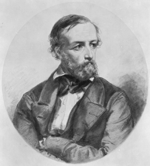
4. Dirichlet and the Modern Definition (1837)
German mathematician Peter Gustav Lejeune Dirichlet completely stripped away the requirement for a formula. He formulated the modern abstract definition: a correspondence where every input value maps to a unique output value. By detaching functions from formulas, Dirichlet made it mathematically necessary to explicitly define the allowed input sets (domains) and output destinations (codomains/ranges).
2. Linear Functions and Monotonicity
The simplest algebraic curve is a straight line. A linear (or affine) function is defined by the formula:
where $m$ and $b$ are given real parameters.
The graph of a linear function is a straight line that passes through the point $(0, b)$ on the $y$-axis:
Monotonicity and Slopes
Functions can be classified by their directional behavior over a domain.
- A function is strictly increasing if for any two arguments $x_1 < x_2$ from the domain, $f(x_1) < f(x_2)$.
- A function is strictly decreasing if for any two arguments $x_1 < x_2$ from the domain, $f(x_1) > f(x_2)$.
- A function is monotone if it is either increasing or decreasing.
A linear function is strictly increasing if $m > 0$ and strictly decreasing if $m < 0$.
Why Monotonicity Guarantees Invertibility
Why do mathematicians care so much whether a function is strictly increasing or decreasing? Because monotonicity guarantees that a function never doubles back on itself.
Think of it like walking down a straight road of houses where every house has a unique address. If a function is strictly increasing, every step you take forward brings you to a higher address. Because the path never loops back, no two different starting distances ($x_1$ and $x_2$) will ever land you at the same house number ($f(x_1) \neq f(x_2)$).
If you arrive at a specific house address (an output), you can trace your steps backward and know uniquely the exact distance you traveled to get there. There are no "collisions" where different paths lead to the same destination.
📈 Theorem: Strict Monotonicity Implies Injectivity (No Collisions)
Proof: Assume $f(x)$ is strictly increasing. If we pick two different inputs $x_1 \neq x_2$, one must be smaller (say, $x_1 < x_2$). Because the function strictly increases, it guarantees that $f(x_1) < f(x_2)$. Since the outputs are unequal, no two inputs ever share a destination. Therefore, the function is injective. $\blacksquare$
The Payoff for Inverses: Why do we care about proving injectivity and surjectivity? Because together, they give us the green light to retrace our steps backward without getting lost.
- No Collisions (Injectivity): Ensures that every house address has a single, unambiguous starting distance. Without this, handing an address to your inverse function would cause a paradox (not knowing whether to point back to $-2$ or $2$).
- No Unreachable Destinations (Surjectivity): Ensures that every house number in our target set actually exists along the road, meaning the inverse function will never hit a blank wall or undefined error.
When a function satisfies both conditions, it forms a perfect bijection. This is what unlocks a clean inverse function $f^{-1}$, allowing us to swap the roles of inputs and outputs and mirror the graph across the diagonal line $y = x$ with total mathematical certainty.
3. Power Functions: The Even/Odd Divide
Now that we understand how straight lines behave, we can step up our algebraic complexity. In calculus and real analysis, we frequently encounter functions where our variable $x$ is multiplied or raised to higher exponents. These are known as power functions, given by the general form $f(x) = x^n$ where $n > 1$ is a natural number.
The term "power" comes directly from the exponent $n$ to which the base variable $x$ is raised. Familiar examples include the squaring function ($f(x) = x^2$) and the cubing function ($f(x) = x^3$). While their algebraic formulas look deceptively simple, their global behavior, graph symmetry, and invertibility radically split depending on whether the exponent $n$ is even or odd.
Even Powers ($n = 2m$)
- Symmetry (Even Functions): $f(-x) = (-x)^{2m} = x^{2m} = f(x)$. Negating the input does not change the output, making the graph mirror-symmetric across the $y$-axis.
- Restricted Range: Because an even power swallows negative signs, outputs can never dip below zero. The range is strictly restricted to $[0, \infty)$.
- The Invertibility Problem: Even powers fail the horizontal line test (e.g., $(-2)^2 = 2^2 = 4$). They suffer from collisions, meaning they are not injective. To build an inverse (like the even root $\sqrt[2m]{x}$), we must artificially restrict the domain to $X = [0, \infty)$ so the curve only moves in one direction.
Odd Powers ($n = 2m + 1$)
- Symmetry (Odd Functions): $f(-x) = (-x)^{2m+1} = -x^{2m+1} = -f(x)$. Negating the input negates the entire output, making the graph point-symmetric with respect to the origin.
- Full Range: Odd powers preserve signs, allowing outputs to span the entire vertical spectrum. Their range is $\mathbb{R}$.
- Naturally Invertible: Odd power functions are strictly increasing across their entire natural domain $\mathbb{R}$. By our monotonicity theorem, this guarantees they have zero collisions (injectivity) naturally. Their inverse, the $(2m+1)$-st root $g(x) = \sqrt[2m+1]{x}$, exists everywhere without needing any domain surgery.
4. Polynomials and Rational Functions
In the previous section, we looked at isolated power functions like $x^2$ and $x^3$. You can think of these pure power functions as mathematical building blocks. By scaling these blocks up or down (scalar multiplication) and stacking them together (addition), we construct polynomial functions.
🧱 Polynomial Primer: Anatomy of an Equation
Before we look at the formal definition, consider a familiar quadratic function:
- Terms: The individual building blocks glued together by plus and minus signs ($3x^2$, $-2x$, and $5$).
- Coefficients: The specific numerical weights attached to each power of $x$ (here, $3$, $-2$, and $5$).
- Degree (or Order): The highest exponent that appears in the equation. Because the highest power here is $x^2$, this is a 2nd-degree polynomial.
Formally, a polynomial function of order (or degree) $n$ generalizes this exact pattern to any number of terms, given by the formula:
where $a_0, \dots, a_n$ are real parameters called the coefficients, and $a_n \neq 0$ is the leading coefficient.
Because these functions only ever involve basic addition, subtraction, and multiplication, they never demand dangerous operations like division by zero or taking the square root of a negative number. Therefore, the natural domain of any polynomial function is the entire set of real numbers, $\mathbb{R}$.
A number $x_0$ from the domain is called a zero or root of the function if $f(x_0) = 0$. Geometrically, these are the points where the graph intersects the $x$-axis. If $x_0$ is a root, the polynomial can be factored cleanly into $f(x) = (x - x_0)g(x)$, which proves that a polynomial of order $n$ has at most $n$ roots.
If polynomial functions are the mathematical equivalent of integers (simple, solid building blocks), then rational functions are the equivalent of fractions. A rational function is formed by taking the ratio (division) of two polynomials:
where $p(x)$ and $q(x)$ are polynomials, and $q(x)$ is not the zero polynomial.
⚠️ The Danger Zone: Division by Zero
Unlike polynomials, which are safe to calculate for any real number, rational functions possess inherent structural weaknesses. If an input $x$ causes the denominator polynomial $q(x)$ to evaluate to zero, the entire function violently breaks down, as division by zero is undefined.
Therefore, the natural domain of a rational function is the set of all real numbers $\mathbb{R}$, strictly excluding the roots of the denominator $q(x)$.
🔄 Worked Example: Finding the Domain
Consider the rational function:
To find the natural domain, we entirely ignore the numerator (the top) and isolate the denominator (the bottom) to find its roots:
- Set the denominator to zero: $x - 2 = 0$
- Solve for $x$: $x = 2$
- Conclusion: The function is valid everywhere except at $x = 2$. Using our interval notation, the natural domain is $(-\infty, 2) \cup (2, \infty)$.
Geometrically, what happens at these excluded points? In most cases, as the $x$-values get closer and closer to the excluded root, the denominator shrinks toward zero, which forces the overall fraction to explode toward infinity (or negative infinity). This creates a sheer, invisible vertical wall on the graph called a vertical asymptote, which the curve approaches but can never cross.
Summary: The Bridge to Calculus
We have officially completed our transition from the discrete mathematics of sequences into the continuous world of functions. This lecture was not just an algebra review; it was about establishing a rigorous, structural vocabulary for the curves we will be manipulating for the rest of the term.
🎓 Key Takeaways from Lecture 7
- Structural Mappings: Functions are rigid rules mapping a domain to a codomain. Identifying the natural domain protects us from algebraic impossibilities (like division by zero or negative roots).
- Invertibility Requires a One-Way Street: Strict monotonicity guarantees injectivity (no collisions), which is the geometric key to unlocking clean inverse functions and safely reflecting graphs across $y = x$.
- Foundational Families: Linear, power, polynomial, and rational functions are the standard building blocks of mathematical modeling. We saw how even/odd exponents dictate symmetry and range, and how rational denominators create impassable vertical asymptotes.
Where does this fit into the overall course?
In Weeks 1 and 2, we built the logical machinery of limits using isolated stepping stones (sequences). Today, we constructed the continuous tracks (functions) that those limits will soon travel along.
Right now, the polynomial and rational curves we defined today are static shapes sitting on a Cartesian plane. But the core of calculus is about dynamic change. In the upcoming lectures, we will take these foundational curves and set them in motion. We will use limits to ask what happens as $x$ gets infinitely close to a dangerous vertical asymptote, and we will build derivatives to measure the exact slope of a power function that is constantly bending.
By securing your understanding of domains, inverses, and asymptotes today, you have just laid the concrete foundation for the calculus we will build tomorrow.
Ready to test your understanding?
Work through the progressive interactive problems to lock in these foundational concepts before moving on to Lecture 8.
Launch Interactive Problem Stepper ➔