Week 3, Lecture 8: Transcendental Functions
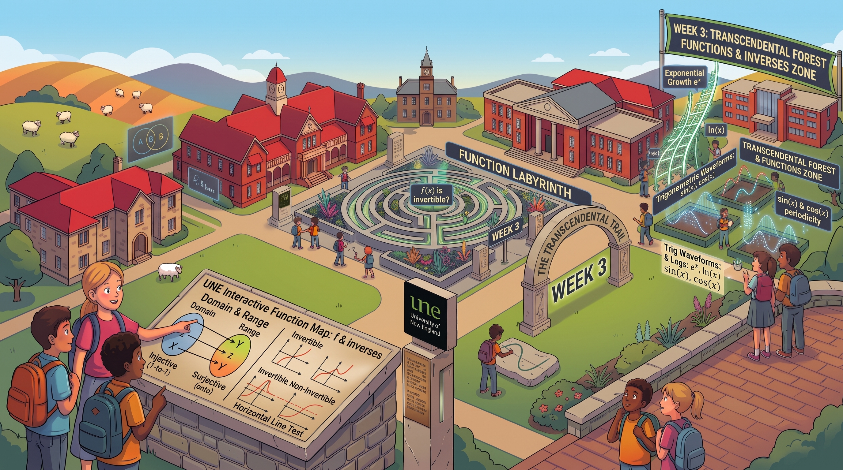
Welcome to Lecture 8: Beyond Algebra
In Lecture 7, we built our foundation on algebraic functions: linear equations, power functions, polynomials, and rational expressions. These are the "building blocks" of early mathematics because they can be computed using a finite sequence of additions, subtractions, multiplications, divisions, and root extractions.
However, nature does not restrict itself to algebra. Sound waves oscillate periodically. Bacteria populations compound and multiply. To model these phenomena, we need a new class of functions that transcend standard polynomial algebra. These are known as Transcendental Functions .
Today, we will formalize exponential growth, demystify the natural logarithm, and establish the geometric and analytical rules governing trigonometric waveforms and their inverses.
📌 Lecture 8 Topics
Beyond Algebra: Napier's Quest, the Ferris Wheel, and Base e
Explore the 16th-century astronomy crisis, John Napier's 20-year secret project to invent logarithms, why calculus requires the "Goldilocks" base $e$, and the geometric reality of the Unit Circle Ferris Wheel.
1. Exponential Functions: From Discrete Steps to Continuous Growth
1.1 The Great Variable Swap: Power vs. Exponential Functions
In Lecture 7, we studied power functions like $f(x) = x^2$ or $f(x) = x^3$. Now, we perform a simple visual swap with massive mathematical consequences: we lock the base in place as a constant and move the variable $x$ up into the exponent.
- Base ($x$): Variable input.
- Exponent ($n$): Fixed constant.
- Growth Mechanism: Additive scaling. Increasing $x$ grows the base of a fixed-dimension geometric shape (like the side of a square $x^2$).
- Base ($a$): Fixed positive constant ($a > 0, a \neq 1$).
- Exponent ($x$): Variable input!
- Growth Mechanism: Multiplicative compounding. Every unit step forward in $x$ multiplies the current height by $a$.
To feel the difference in your bones, compare $x^2$ (power) against $2^x$ (exponential) as $x$ grows:
| Input $x$ | $1$ | $2$ | $3$ | $4$ | $5$ | $10$ | $20$ |
|---|---|---|---|---|---|---|---|
| Power ($x^2$) | $1$ | $4$ | $9$ | $16$ | $25$ | $100$ | $400$ |
| Exponential ($2^x$) | $2$ | $4$ | $8$ | $16$ | $32$ | $1{,}024$ | $1{,}048{,}576$ |
1.2 The Conceptual Puzzle: What Does $2^{\sqrt{2}}$ Actually Mean?
Here is the question that confuses almost everyone when they first study analysis: If an exponent tells us how many times to multiply a number by itself, how on earth can we raise $a$ to a fraction, a negative number, or an irrational number like $\pi$? You cannot multiply $2$ by itself $\sqrt{2}$ times!
In Week 1, we studied geometric sequences $a_n = a^n$, which only existed as isolated dots at integer steps $n = 1, 2, 3, \dots$. To turn those isolated stepping stones into a smooth, unbroken curve across the entire real line $\mathbb{R}$, mathematics builds a four-stage bridge , demanding at each stage that the fundamental rule $a^{x+y} = a^x \cdot a^y$ never breaks:
This is our Week 1 geometric sequence. $a^1 = a$, $a^2 = a \cdot a$, and $a^n = \underbrace{a \cdot a \cdots a}_{n \text{ times}}$. Taking one step right ($n \to n+1$) multiplies the value by $a$.
If stepping right ($+1$) multiplies by $a$, then stepping left ($-1$) must divide by $a$. Starting at $a^1 = a$ and stepping left to $x = 0$ gives $a^0 = \frac{a}{a} = 1$. Stepping left again to $x = -1$ gives $a^{-1} = \frac{1}{a}$, and $n$ steps left gives $a^{-n} = \frac{1}{a^n}$. Crucial takeaway: A negative exponent does not make the output negative—it simply flips the base into a fraction!
What is $a^{1/2}$? It is the halfway stepping stone between $x = 0$ and $x = 1$. If two half-steps make one full step, then multiplying $a^{1/2}$ by itself must equal a single full step of $a^1$: $$a^{1/2} \cdot a^{1/2} = a^{1/2 + 1/2} = a^1 = a \implies a^{1/2} = \sqrt{a}$$ In general, $a^{1/q} = \sqrt[q]{a}$ (the unique positive $q$-th root of $a$), and $a^{p/q} = (\sqrt[q]{a})^p$.
How do we compute $2^{\sqrt{2}}$? Here is where Weeks 1 & 2 pay off ! Even though $\sqrt{2} = 1.4142135\dots$ is irrational, we can trap it with a sequence of rational decimals: $q_1 = 1.4$, $q_2 = 1.41$, $q_3 = 1.414, \dots$. Since each $q_n$ is a fraction, $2^{q_n}$ is already defined by Stage 3! Because the sequence $2^{1.4}, 2^{1.41}, 2^{1.414}, \dots$ is monotonic and bounded, the Monotone Convergence Theorem guarantees it converges to a unique real limit, which we define as $2^{\sqrt{2}}$: $$a^x = \lim_{n \to \infty} a^{q_n} \quad \text{where } (q_n) \subset \mathbb{Q} \text{ and } q_n \to x$$
1.3 The Rules of the Base: Why Must $a > 0$ and $a \neq 1$?
Every textbook states that an exponential function $f(x) = a^x$ requires a base $a > 0$ with $a \neq 1$. These aren't arbitrary rules made up to annoy you—if you violate them, the continuous curve shatters:
- Why $a < 0$ is forbidden (The Imaginary Swiss Cheese): Suppose you tried to use a negative base, like $f(x) = (-2)^x$. What happens at $x = \frac{1}{2}$? You get $(-2)^{1/2} = \sqrt{-2}$, which does not exist in the real numbers $\mathbb{R}$! The graph would be punctured with infinitely many holes at every fraction with an even denominator ($\frac{1}{2}, \frac{1}{4}, \frac{3}{4}, \dots$).
- Why $a = 0$ is forbidden (Division by Zero): If $a = 0$, then for any negative input like $x = -2$, we would have $0^{-2} = \frac{1}{0^2} = \frac{1}{0}$, which is undefined.
- Why $a = 1$ is excluded (The Flatline): Since $1^x = 1$ for every real number $x$, the function $f(x) = 1^x$ is just a horizontal constant line. Because it is completely flat, it fails the Horizontal Line Test (it is not injective) and has no inverse!
1.4 The Algebraic Engine: Translating Addition into Multiplication
The secret superpower of exponential functions is that they act as a bridge between two operations: they turn addition in the input (domain) into multiplication in the output (range) . For any $a, b > 0$ and any $x, y \in \mathbb{R}$:
| Law Name | Algebraic Identity | What It Means Geometrically on the Graph |
|---|---|---|
| Zero Exponent | $a^0 = 1$ | Universal Anchor: Every pure exponential graph $y = a^x$ passes through the exact same $y$-intercept at $(0, 1)$. |
| Addition-to-Product | $a^{x+y} = a^x \cdot a^y$ | Shifting right by $+y$ units along the $x$-axis scales the vertical height of the curve by a factor of $a^y$. |
| Reciprocal / Mirror | $a^{-x} = \frac{1}{a^x} = \left(\frac{1}{a}\right)^x$ | Mirror Reflection: Replacing $x$ with $-x$ reflects the graph across the $y$-axis. Thus, $(1/2)^x$ is the exact mirror image of $2^x$! |
| Subtraction-to-Quotient | $a^{x-y} = \frac{a^x}{a^y}$ | Shifting left by $y$ units divides the vertical height by $a^y$. |
| Power of a Power | $(a^x)^y = a^{xy}$ | Changing the base from $a$ to $a^y$ is identical to horizontally compressing/stretching the input $x$ by $y$. |
1.5 The Two Regimes: Exponential Growth ($a > 1$) vs. Decay ($0 < a < 1$)
Depending on whether your base $a$ is larger than $1$ or a fraction between $0$ and $1$, the exponential function splits into two mirror-image behaviors:
Regime 1: Exponential Growth ($a > 1$)
Example: $f(x) = 2^x$ — Strictly Increasing
- Left Tail ($x \to -\infty$): Approaches the horizontal asymptote $y = 0$ (never touches or crosses $0$).
- Right Tail ($x \to +\infty$): Explodes to $+\infty$.
- Monotonicity: Strictly increasing ($x_1 < x_2 \implies a^{x_1} < a^{x_2}$).
Regime 2: Exponential Decay ($0 < a < 1$)
Example: $f(x) = \left(\frac{1}{2}\right)^x = 2^{-x}$ — Strictly Decreasing
- Left Tail ($x \to -\infty$): Explodes to $+\infty$.
- Right Tail ($x \to +\infty$): Decays toward the horizontal asymptote $y = 0$.
- Monotonicity: Strictly decreasing ($x_1 < x_2 \implies a^{x_1} > a^{x_2}$).
🔑 Connecting to Lecture 7: Domain, Range, and Bijection
- Natural Domain: $\mathbb{R} = (-\infty, \infty)$. You can plug any real number into an exponential function without fear of dividing by zero or taking even roots of negative numbers.
- Range (Image): $(0, \infty) = \mathbb{R}^+$. Because the base $a > 0$, raising it to any real power always produces a strictly positive number ($a^x > 0$). An exponential function can never equal zero and can never be negative!
- Injectivity & Invertibility: Because $f(x) = a^x$ is strictly monotonic (strictly increasing for $a > 1$, strictly decreasing for $0 < a < 1$), it passes the Horizontal Line Test everywhere. When we restrict its codomain to its range $(0, \infty)$, $f: \mathbb{R} \to (0, \infty)$ is a perfect bijection —which guarantees that its inverse function (the logarithm in Section 2!) exists!
1.6 Euler's Number $e$: Why Calculus Prefers $e^x$ Over $2^x$ or $10^x$
Out of all possible bases $a > 1$, there is one special irrational number that serves as the natural currency of calculus: Euler's number $e \approx 2.718281828\dots$ .
Where does $e$ come from? Recall from Week 2 (Lecture 5) that we proved the sequence $a_n = \left(1 + \frac{1}{n}\right)^n$ is strictly increasing and bounded above by $3$. By the Monotone Convergence Theorem, its limit defines $e$:
1.6 Euler's Number $e$: Why Calculus Prefers $e^x$ Over $2^x$ or $10^x$
Out of all possible bases $a > 1$, there is one special irrational number that serves as the natural currency of calculus: Euler's number $e \approx 2.718281828\dots$ .
Where does $e$ come from? Recall from Week 2 (Lecture 5) that we proved the sequence $a_n = \left(1 + \frac{1}{n}\right)^n$ is strictly increasing and bounded above by $3$. By the Monotone Convergence Theorem, its limit defines $e$:
The Geometric Secret of $e^x$: The Search for the Perfect Slope
Every exponential curve $y = a^x$ behaves geometrically the exact same way at the $y$-axis: it passes through the universal anchor point $(0, 1)$. However, each base crosses that point at a uniquely different steepness (slope). If you zoom in infinitely close to $(0,1)$, the curve looks like a straight line. The steepness of that line depends entirely on the base $a$.
- Base $2$ is too slow: If you graph $y = 2^x$, the slope of the curve as it crosses $(0, 1)$ is slightly flat, measuring approximately $0.693$.
- Base $3$ is too fast: If you graph $y = 3^x$, the curve climbs more aggressively. Its slope at $(0, 1)$ is slightly too steep, measuring approximately $1.099$.
- Base $e$ is the "Goldilocks" Base: The irrational number $e \approx 2.718$ is the precise, perfect balance point between $2$ and $3$. The curve $y = e^x$ crosses $(0, 1)$ at a pristine $45^\circ$ angle, giving it a slope of exactly $1$ .
If the slope of $y = e^x$ at $x = 0$ is exactly $1$, a beautiful mathematical chain reaction occurs. Because exponential functions turn addition into multiplication ($e^{x+h} = e^x \cdot e^h$), the slope at any other point on the curve is just the slope at zero scaled up by the height of the curve.
Since the baseline slope is $1$, scaling it by $e^x$ just gives you $e^x$. This creates the ultimate property of the natural exponential function: At every single point on the curve $y = e^x$, the exact steepness of the slope is completely equal to its current vertical height!
This property—where the rate of growth is identical to the amount currently present ($y' = y$)—is the holy grail of differential equations. It is why $e$ governs radioactive decay, bacterial population modeling, and continuously compounding interest. You can model these phenomena using base $2$ or base $10$, but you will constantly have to multiply your equations by messy corrective constants (like $\ln(2) \approx 0.693$). By using base $e$, the mathematics becomes perfectly clean.
Interactive Simulator: Hunting the Golden Base
What Is Happening
Why The System Does This
🎯 Worked Examples: Mastering Exponential Equations & Inequalities
Example 1 (Solving by Common Base Reduction): Solve $9^{x-1} = \frac{1}{27}$ for $x$.
- Spot the common prime base: Both $9$ and $27$ are powers of $3$ ($9 = 3^2$ and $27 = 3^3$).
- Rewrite both sides with base $3$: $$(3^2)^{x-1} = \frac{1}{3^3} \implies 3^{2(x-1)} = 3^{-3} \implies 3^{2x - 2} = 3^{-3}$$
- Use injectivity (one-to-one property): Because $f(t) = 3^t$ is strictly increasing, two outputs are equal if and only if their exponents are equal: $$2x - 2 = -3 \implies 2x = -1 \implies x = -\frac{1}{2}.$$
Example 2 (The Decay Inequality Trap): Solve $\left(\frac{1}{2}\right)^{x-3} > \frac{1}{8}$ for $x$.
- Express with the same base: Since $\frac{1}{8} = \left(\frac{1}{2}\right)^3$, the inequality becomes: $$\left(\frac{1}{2}\right)^{x-3} > \left(\frac{1}{2}\right)^3$$
- Watch the monotonicity direction! Because the base $a = \frac{1}{2}$ satisfies $0 < a < 1$, the function is strictly decreasing . Larger outputs come from smaller exponents! Therefore, stripping the base flips the inequality sign : $$x - 3 < 3 \implies x < 6.$$
2. Logarithmic Functions and Base $e$: Running Exponents in Reverse
2.1 The Historical Origins of Logarithms: Napier's 20-Year Quest
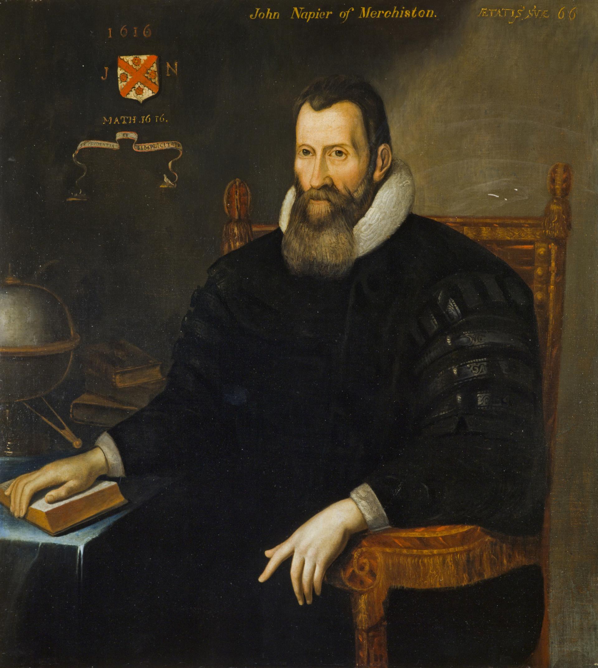

Before calculators, computers, or even the widespread use of decimals, astronomers and navigators calculated the positions of stars, planets, and ocean trade routes entirely by hand. During the late 16th century, figures like Johannes Kepler faced a massive astronomical crisis: tracking planetary orbits required multiplying and dividing multi-digit numbers with extreme precision. Doing 8-digit multiplication by hand took days, and a single arithmetic error meant months of calculations had to be discarded. Scientists desperately needed a shortcut to turn brutal multiplication into simple addition.
Enter John Napier , the eighth Laird of Merchiston, a Scottish landowner, theologian, and mathematician. Napier spent roughly twenty years in secret working on a way to simplify calculation. He understood a fundamental principle of exponents: multiplying numbers is the same as adding their exponents (for example, $10^2 \times 10^3 = 10^{2+3} = 10^5$).
The word logarithm was coined by John Napier from two Greek words: logos , meaning ratio or proportion, and arithmos , meaning number. Literally translated, a logarithm is a "ratio-number." Napier chose this name because his original mathematical tables were designed to track how geometric ratios (like the proportional steps of a scaling sequence) corresponded to equal arithmetic steps (counting numbers). By turning the relationship between multiplying ratios into a running index of numbers, he created a system where adding the "ratio-numbers" together gave the exact equivalent of multiplying the underlying values.
In 1614, Napier published his breakthrough masterpiece at his own expense— Mirifici Logarithmorum Canonis Descriptio ("A Description of the Admirable Table of Logarithms"). Working entirely without modern algebraic notation, Napier spent years calculating these values by hand using a geometric model of moving points.
Napier's tables did not feature logarithms in the modern Base 10 or Base $e$ sense; rather, they used a decaying proportional scale that mapped geometric sequences to arithmetic sequences. The book contained a brief introduction explaining how to use the tables to turn complex multiplication and division into simple addition and subtraction, followed by dozens of pages of dense calculation tables that changed European science forever.
Shortly after Napier's book appeared, the English mathematician Henry Briggs , a professor at Gresham College in London, was so profoundly struck by the discovery that he rode on horseback all the way to Edinburgh to meet Napier in person. During their historic 1615 and 1616 meetings, Briggs suggested shifting from Napier's original system to a much more intuitive decimal baseline where $\log_{10}(1) = 0$ and $\log_{10}(10) = 1$. Napier warmly endorsed the proposal.
Briggs took on the staggering computational burden of calculating these new tables by hand, eventually publishing his monumental work Arithmetica Logarithmica in 1624. It contained common logarithms for numbers from 1 to 20,000 and from 90,000 to 100,000, calculated out to an astonishing 14 decimal places.
These Base 10 tables became an instant international sensation. The great astronomer Johannes Kepler used them to complete his definitive Rudolphine Tables , revolutionizing celestial mechanics. Centuries later, the French mathematician Pierre-Simon Laplace famously observed that logarithms, by shortening the exhausting labor of manual calculation, "doubled the life of the astronomer," allowing science, engineering, and global navigation to flourish centuries before the invention of electronic computers.
2.2 Demystifying the Logarithm: The "Exponent Hunter"
For many students, the word $\log$ triggers an instant mental block. To strip away the mystery, memorize this single sentence: a logarithm is just an exponent .
In Section 1, we saw that an exponential function $f(x) = a^x$ takes an exponent $x$ as its input and outputs a scaled number $y$. But what if we know the final scaled number $y$, and we need to hunt down the hidden exponent $x$ that produced it? That "exponent hunter" is the logarithm.
In Lecture 7, we proved that any strictly monotonic function is injective (one-to-one) and therefore possesses a unique inverse function. Because $f: \mathbb{R} \to (0, \infty)$ defined by $f(x) = a^x$ ($a > 0, a \neq 1$) is strictly monotonic and surjective onto $(0, \infty)$, it is a perfect bijection . Its inverse function $f^{-1}: (0, \infty) \to \mathbb{R}$ is called the logarithm with base $a$ , written $\log_a(x)$.
For any base $a > 0$ ($a \neq 1$), any positive number $x \in (0, \infty)$, and any real number $y \in \mathbb{R}$:
How to read $\log_a(x)$ in plain English: Whenever you see $\log_a(x)$, translate it in your head as the question: "To what power must I raise the base $a$ in order to get $x$?"
- $\log_2(8) = 3 \quad$ because $2^3 = 8$. ("What power of $2$ gives $8$? Answer: $3$.")
- $\log_{10}\left(\frac{1}{100}\right) = -2 \quad$ because $10^{-2} = \frac{1}{100}$.
- $\log_5(1) = 0 \quad$ because $5^0 = 1$.
- $\log_9(3) = \frac{1}{2} \quad$ because $9^{1/2} = \sqrt{9} = 3$.
2.3 Mutual Annihilation & The Strict Domain Barrier ($x > 0$)
Because $f(x) = a^x$ and $f^{-1}(x) = \log_a(x)$ are exact inverse functions, applying one immediately after the other cancels both operations out, leaving your original input untouched. However, you must pay close attention to which inputs are legal in each direction:
"To what power must I raise $a$ to get $a^x$?" Obviously $x$! Because $a^x$ is always positive for any real $x$, this identity works for all real numbers $x \in \mathbb{R}$ .
Raising $a$ to "the power that turns $a$ into $x$" produces $x$! Because $x$ is fed into $\log_a(x)$ first, this identity is strictly restricted to positive numbers $x > 0$ .
⚠️ The #1 Domain Trap in Calculus: Why $\log_a(0)$ and $\log_a(-5)$ Do Not Exist
In Lecture 7, we learned that when you invert a function, the Domain and Range swap places :
Because $a^y > 0$ for every real $y$, there is no exponent $y$ in the universe that can make $a^y = 0$ or $a^y = -5$. Therefore, you can NEVER feed zero or a negative number into a logarithm! Whenever you see $\log_a(\text{expression})$, your immediate reflex must be to set up the strict domain guard: $\text{expression} > 0$.
2.4 Geometric Mirroring: Reflecting Across $y = x$
As we established in Lecture 7, the graph of any inverse function $f^{-1}(x)$ is obtained by reflecting the original graph $f(x)$ across the diagonal mirror line $y = x$. Every coordinate pair $(u, v)$ on $y = a^x$ swaps to become $(v, u)$ on $y = \log_a(x)$:
- The universal exponential $y$-intercept $(0, 1)$ flips to become the universal logarithmic $x$-intercept $(1, 0)$ .
- The exponential base landmark $(1, a)$ flips to become $(a, 1)$ .
- The exponential horizontal asymptote $y = 0$ (as $x \to -\infty$) flips to become a vertical asymptote $x = 0$ (the $y$-axis, where $\log_a(x) \to -\infty$ as $x \to 0^+$ for $a > 1$).
Base $a > 1$: Mirror Reflection
$y = 2^x$ and $y = \log_2(x)$ across $y = x$
- Strictly Increasing: For $a > 1$, $x_1 < x_2 \implies \log_a(x_1) < \log_a(x_2)$.
- Near Zero ($x \to 0^+$): Plunges to $-\infty$ along the vertical wall $x = 0$.
- Right Tail ($x \to +\infty$): Grows to $+\infty$, but extremely slowly .
Base $0 < a < 1$: Strictly Decreasing
$y = \log_{1/2}(x) = -\log_2(x)$
- Strictly Decreasing: For $0 < a < 1$, $x_1 < x_2 \implies \log_a(x_1) > \log_a(x_2)$.
- Near Zero ($x \to 0^+$): Shoots up to $+\infty$ along $x = 0$.
- Sign Rule: Positive for $0 < x < 1$, zero at $x = 1$, negative for $x > 1$.
2.5 The Algebraic Laws of Logarithms: Translating Exponents
If you have ever felt intimidated or completely lost when looking at logarithm rules, take a deep breath. You are completely normal, and you are in exactly the right place. These laws often look like an alien language of shifting letters and arbitrary rules. But here is the comforting truth: you already know these laws.
Remember our golden rule from Section 2.1: a logarithm is just an exponent . Therefore, every single "Logarithm Law" is simply an old, familiar "Exponent Law" written from a different perspective. Back in 1614, mathematicians realized that if they converted giant, messy numbers into their exponents (their logarithms), they could do complex arithmetic much faster. Let's walk through exactly how this works, step by step.
1. The Product Law: Turning Multiplication into Addition
The Intuition (The "Exponent Detector"): Think of a logarithm as an "exponent detector." When you feed a number into a logarithm, it strips away the base and hands you back just the exponent. To see why this law works, let's look at how you naturally multiply numbers using base 10:
- The raw numbers: Imagine you want to multiply $100 \times 1,000$.
- The exponent view: You already know that $100$ is $10^2$ (its exponent is $2$), and $1,000$ is $10^3$ (its exponent is $3$).
- The multiplication step: When you multiply $10^2 \times 10^3$, you don't actually multiply the exponents together. You just add them together to get $10^5$ (which is $100,000$). The absolute golden rule for exponents is that multiplying the bases means adding their exponents ($2 + 3 = 5$).
- The logarithm view: Because a logarithm is just a tool that isolates the exponent, it obeys that exact same rule. If you ask a base-10 logarithm to find the exponent of $(100 \times 1,000)$, it finds the exponent of $100$, finds the exponent of $1,000$, and adds them together!
Written out in mathematical notation, that exact thought process looks like this:
Locking in the Mechanism with Base 2: Let's trace this exact same logic with base 2 to prove it isn't just a base-10 trick. Suppose we want to multiply $8 \times 4$.
- The Exponents: We know $8 = 2^3$ and $4 = 2^2$.
- The Logarithms: Therefore, $\log_2(8) = 3$ and $\log_2(4) = 2$.
- The Product: If we multiply the raw numbers, $8 \times 4 = 32$. If we count our powers of two ($2, 4, 8, 16, 32$), we know that $32$ is $2^5$. Therefore, its logarithm is $5$.
- The Law in Action: Does adding the individual exponents give us the exact exponent of the total? Yes! $3 + 2 = 5$.
The mathematical translation for Base 2:
2. The Quotient Law: Turning Division into Subtraction
The Intuition (The "Exponent Detector" strikes again): Just as multiplication forces you to add exponents, division forces you to subtract them. Let's look at how division works with our familiar base 10:
- The raw numbers: Imagine you want to divide $100,000 \div 100$.
- The exponent view: You know that $100,000$ is $10^5$ (its exponent is $5$), and $100$ is $10^2$ (its exponent is $2$).
- The division step: When you calculate $\frac{10^5}{10^2}$, you don't actually do long division. You just subtract the bottom exponent from the top exponent to get $10^3$ (which is $1,000$). The golden rule here is that dividing the bases means subtracting their exponents ($5 - 2 = 3$).
- The logarithm view: Once again, our "exponent detector" does exactly what you just did in your head. To find the exponent of a division problem, it finds the exponent of the top number, finds the exponent of the bottom number, and subtracts them!
Written out in mathematical notation, that exact thought process looks like this:
Locking in the Mechanism with Base 2: Let's prove this works exactly the same way for base 2. Suppose we want to divide $32 \div 4$.
- The Exponents: We know $32 = 2^5$ and $4 = 2^2$.
- The Logarithms: Therefore, $\log_2(32) = 5$ and $\log_2(4) = 2$.
- The Quotient: If we divide the raw numbers, $32 \div 4 = 8$. We know that $8$ is $2^3$. Therefore, its logarithm must be $3$.
- The Law in Action: Does subtracting the individual exponents give us the exact exponent of the result? Yes! $5 - 2 = 3$.
The mathematical translation for Base 2:
3. The Power Law (The "Pull-Down" Trick): Turning Powers into Multipliers
The Intuition (Repeated Addition): This is arguably the most powerful tool in all of pre-calculus because it rescues variables trapped up in the exponent and drops them down to the ground floor as normal multipliers. To see why this is totally legal, let's use base 10 and look at $100^3$:
- The expanded view: You already know that $100^3$ literally just means $100 \times 100 \times 100$.
- Using the Product Law: Based on Law 1, we know our "exponent detector" turns multiplication into addition. So, $\log_{10}(100 \times 100 \times 100)$ becomes $\log_{10}(100) + \log_{10}(100) + \log_{10}(100)$.
- The shortcut: What is the mathematical shortcut for adding the exact same thing three times? Multiplying by 3! Since $\log_{10}(100)$ is $2$, adding $2 + 2 + 2$ is just $3 \times 2$.
- The pull-down trick: Instead of writing all that expansion out, you can just grab the exponent $3$, pull it down to the front of the logarithm, and multiply.
Written out in mathematical notation, the pull-down trick looks like this:
Locking in the Mechanism with Base 2: Let's verify this trick with base 2 to prove it works universally. Suppose we want to find the logarithm of $8^2$.
- The manual way: First, calculate the power. $8^2 = 64$. Now, what power of $2$ gives $64$? If we count our powers of two ($2, 4, 8, 16, 32, 64$), we find it is $2^6$. So the true exponent is $6$.
- The pull-down way: Instead of bothering to figure out that $8^2$ is $64$, we just pull the $2$ down to the front: $2 \times \log_2(8)$.
- The result: We already know $\log_2(8)$ is $3$ (since $2^3 = 8$). So we just multiply $2 \times 3$, which gives us $6$ instantly!
The mathematical translation for Base 2:
4. The Reciprocal Flip: Fractions are just Negative Exponents
The Intuition (The Power Law Shortcut): This law isn't actually a new rule at all—it is just an incredibly useful shortcut built directly from the Power Law we just learned.
- The fraction view: Remember from Section 1.2 that a negative exponent just means "divide by the base." So, writing the fraction $\frac{1}{100}$ is mathematically identical to writing $100^{-1}$.
- The pull-down step: If we ask our exponent detector for $\log_{10}\left(\frac{1}{100}\right)$, we can just rewrite it as $\log_{10}(100^{-1})$. Now, use the Power Law! We grab that $-1$ and pull it down to the front: $-1 \cdot \log_{10}(100)$.
- The result: The logarithm of a fraction is exactly the same thing as the negative logarithm of the flipped whole number! Since $\log_{10}(100)$ is $2$, the answer is simply $-2$.
Written out in mathematical notation, that exact thought process looks like this:
Locking in the Mechanism with Base 2: Let's verify this trick with base 2. Suppose you are in an exam and need to find the logarithm of the fraction $\frac{1}{8}$.
- The manual way: What power of $2$ gives $\frac{1}{8}$? We know $2^3 = 8$, so to force the $8$ into the denominator, the exponent must be negative: $2^{-3} = \frac{1}{8}$. The true exponent is $-3$.
- The flip trick: Instead of doing that mental gymnastics and worrying about negative fractions, just flip the fraction upside down and stick a negative sign in front: $-\log_2(8)$.
- The result: We already know $\log_2(8)$ is $3$. Throwing the negative sign on it gives us $-3$ instantly!
The mathematical translation for Base 2:
When you are first learning this, it is very tempting to "invent" math rules that look correct but are totally false. Logarithms do not behave like standard multiplication, so you cannot "distribute" them across a bracket.
- $\log_a(x + y)$ DOES NOT EQUAL $\log_a(x) + \log_a(y)$. (You cannot distribute a log over addition).
- $\frac{\log_a(x)}{\log_a(y)}$ DOES NOT EQUAL $\log_a(x - y)$. (A fraction of two logs is not subtraction).
2.6 The Natural Logarithm ($\ln x$) and the Change of Base Formula
Just as $e^x$ is the natural exponential function of calculus, its inverse function—the logarithm with base $e$—is called the natural logarithm and is given its own dedicated shorthand notation:
Why does $\ln(x)$ rule calculus? Remember from Section 1.6 that $y = e^x$ crosses $(0, 1)$ with a clean slope of $1$. Because $y = \ln(x)$ is the mirror reflection of $y = e^x$ across $y = x$, $y = \ln(x)$ crosses its $x$-intercept $(1, 0)$ with a clean slope of $1$ ! In differential calculus, its derivative is simply $\frac{d}{dx}[\ln(x)] = \frac{1}{x}$, with no messy scaling constants attached.
The Change of Base Formula: Why You Only Ever Need One Logarithm
In standard mathematics and programming, you are frequently handed logarithms in strange bases, like $\log_2(32)$ or $\log_7(50)$. The problem is that calculus only plays nicely with the natural base $e$. Furthermore, your physical calculator and standard programming libraries typically only compute the natural logarithm ($\ln$) or the common logarithm ($\log_{10}$).
To evaluate a strange base, you have to translate it into a language your tools understand. The Change of Base formula allows you to rip out the old, awkward base and replace it with any new base you want. Because calculus demands base $e$, we almost exclusively convert things into natural logarithms ($\ln$). Here is a remarkable fact: every logarithm $\log_a(x)$, regardless of its base $a$, is just a vertically scaled copy of the natural logarithm $\ln(x)$!
For any valid bases $a, b > 0$ ($a, b \neq 1$) and any $x > 0$:
Visual Mnemonic: Look at the original expression $\log_a(x)$. The target number $x$ is written normally, but the base $a$ is written as a subscript, physically lower down. When you apply the formula, that physical relationship stays exactly the same: the $x$ stays on top in the numerator ($\ln(x)$), and the base $a$ goes down into the basement (the denominator: $\ln(a)$).
3-Step Proof (Using Exponents):
1. Let $y = \log_a(x)$. By the Rosetta Stone equivalence, this means $a^y = x$.
2. Take the natural logarithm $\ln(\cdot)$ of both sides: $\ln(a^y) = \ln(x)$.
3. Apply the Power Pull-Down Rule ($y \ln(a) = \ln(x)$) and divide by $\ln(a) \neq 0$ to get $y = \frac{\ln(x)}{\ln(a)}$. $\blacksquare$
This formula is also how we rewrite any exponential $a^x$ in terms of the natural base $e$: since $a = e^{\ln(a)}$, raising both sides to the power $x$ gives the universal calculus identity:
🎯 Worked Examples: Logarithmic Domains, Equations & Inverses
Example 1 (Converting to Compute a Value): Calculate $\log_2(8)$ using the Change of Base formula.
- Use the basement trick: Rewrite it using natural logs: $$\log_2(8) = \frac{\ln(8)}{\ln(2)}$$
- Simplify the numerator: Since $8 = 2^3$, we can rewrite the top: $$\frac{\ln(2^3)}{\ln(2)}$$
- Apply the Power Law: Pull the $3$ down to the front: $$\frac{3 \cdot \ln(2)}{\ln(2)}$$
- Cancel: The $\ln(2)$ terms cancel out perfectly, leaving exactly $3$ .
Example 2 (The Calculus Prep): Prepare the function $f(x) = \log_5(x)$ for differentiation.
- Calculus formulas do not work on base $5$. Before you do any calculus, use the Change of Base formula to rewrite the function: $$f(x) = \frac{\ln(x)}{\ln(5)}$$
- Because $\ln(5)$ is just a constant number, this is the exact same thing as writing $f(x) = \left(\frac{1}{\ln 5}\right) \cdot \ln(x)$. Now it is a standard natural logarithm that you can easily differentiate!
Example 3 (Finding the Natural Domain of a Composite Logarithm): Find the natural domain of $f(x) = \ln(x^2 - 9)$.
- Set up the strict domain guard: The argument inside $\ln(\cdot)$ must be strictly positive: $$x^2 - 9 > 0 \implies (x - 3)(x + 3) > 0$$
- Analyze the sign of the parabola: The quadratic $x^2 - 9$ crosses zero at $x = -3$ and $x = 3$, and is positive outside its roots (where $x < -3$ or $x > 3$).
- Natural Domain: $(-\infty, -3) \cup (3, \infty)$. (Notice that $[-3, 3]$ is completely excluded!)
Example 4 (Solving a Logarithmic Equation & Checking for Extraneous Roots): Solve $\log_2(x) + \log_2(x - 2) = 3$.
- Establish the domain first! Both $\log_2(x)$ and $\log_2(x-2)$ must be valid, requiring $x > 0$ and $x - 2 > 0$. Thus, any valid solution must satisfy $x > 2$ .
- Consolidate using the Product-to-Sum Law: $$\log_2\big(x(x - 2)\big) = 3$$
- Unlock the logarithm using the Rosetta Stone ($y = \log_2(\dots) \iff 2^y = \dots$): $$x(x - 2) = 2^3 = 8 \implies x^2 - 2x - 8 = 0 \implies (x - 4)(x + 2) = 0$$
- Filter against the domain guard ($x > 2$): The candidate $x = -2$ fails because $\log_2(-2)$ is undefined! Only $x = 4$ survives.
Example 5 (Inverting a Shifted Exponential Function): Find the inverse $f^{-1}(x)$ of $f(x) = 3 \cdot e^{2x - 1} + 5$.
- Set $y = f(x)$ and isolate the exponential term $e^{2x-1}$: $$y = 3e^{2x - 1} + 5 \implies y - 5 = 3e^{2x - 1} \implies e^{2x - 1} = \frac{y - 5}{3}$$
- Apply $\ln(\cdot)$ to both sides to annihilate the base $e$: $$\ln\left(e^{2x - 1}\right) = \ln\left(\frac{y - 5}{3}\right) \implies 2x - 1 = \ln\left(\frac{y - 5}{3}\right)$$
- Solve for $x$ and swap variables: $$x = \frac{1}{2}\left(1 + \ln\left(\frac{y - 5}{3}\right)\right) \implies f^{-1}(x) = \frac{1}{2} + \frac{1}{2}\ln\left(\frac{x - 5}{3}\right), \quad \text{with domain } (5, \infty).$$
3. Trigonometric Functions: Sine and Cosine (From Zero to Calculus)
3.1 Why Do We Need Trigonometry in Calculus?
Look at every family of functions we have studied so far—linear, polynomial, rational, exponential, and logarithmic. As $x$ marches toward $+\infty$, every single one of them either explodes to infinity, plunges to negative infinity, or flattens out against a horizontal asymptote. None of them can repeat themselves.
Yet the physical universe is full of things that cycle over and over: pendulums swinging, alternating electrical currents, sound waves, ocean tides, and planets orbiting stars. To model repeating cycles mathematically, we need periodic functions . And the simplest repeating motion in geometry is walking around a circle .
3.2 First Principles: What is a Radian, and Why Does Calculus Ban Degrees?
If you have heard of angles in everyday life, you have probably heard of degrees ($360^\circ$ in a full circle, $90^\circ$ in a right corner). Where did the number $360$ come from? Ancient Babylonian astronomers chose $360$ because it divides cleanly by $2, 3, 4, 5, 6, 8, 9, 10, 12$, and is close to the $365$ days in a year.
In calculus, however, $360^\circ$ is a completely arbitrary human convention—it has no intrinsic connection to the size of a circle. If we want to do calculus on a function $f(x)$, the input $x$ and the output $f(x)$ must be measured in the exact same pure real-number units (lengths!). This is why calculus uses radians .
Draw a circle of radius $r = 1$ centered at the origin $(0,0)$. We call this the Unit Circle ($x^2 + y^2 = 1$).
Now, stand at the rightmost point $(1, 0)$ and start walking along the curved rim of the circle. An angle of $x$ radians is literally the physical distance $x$ you have walked along the rim of the unit circle!
- Positive angle ($x > 0$): Walk counter-clockwise (up and around) a distance of $x$.
- Negative angle ($x < 0$): Walk clockwise (down and around) a distance of $|x|$.
- Full Circle ($2\pi$ radians): The circumference of a circle is $C = 2\pi r$. Since our radius is $r = 1$, walking all the way around the unit circle once is a distance of $2\pi \approx 6.283$ units . Therefore, $360^\circ = 2\pi\text{ radians}$!
- Half Circle ($\pi$ radians): Walking halfway around the circle to $(-1, 0)$ is a distance of $\pi \approx 3.14159$ units ($180^\circ = \pi\text{ radians}$).
| Fraction of a Circle | Zero | $\frac{1}{12}$ Turn | $\frac{1}{8}$ Turn | $\frac{1}{6}$ Turn | Quarter Turn | Half Turn | $\frac{3}{4}$ Turn | Full Turn |
|---|---|---|---|---|---|---|---|---|
| Degrees ($^\circ$) | $0^\circ$ | $30^\circ$ | $45^\circ$ | $60^\circ$ | $90^\circ$ | $180^\circ$ | $270^\circ$ | $360^\circ$ |
| Radians (Arc Length $x$) | $0$ | $\frac{\pi}{6}$ | $\frac{\pi}{4}$ | $\frac{\pi}{3}$ | $\frac{\pi}{2}$ | $\pi$ | $\frac{3\pi}{2}$ | $2\pi$ |
Conversion Formula: Since $\pi\text{ radians} = 180^\circ$, multiply degrees by $\frac{\pi}{180}$ to get radians, and multiply radians by $\frac{180}{\pi}$ to get degrees.
3.3 Defining Cosine and Sine: Your $(x, y)$ GPS Coordinates on the Unit Circle
Forget complicated triangle acronyms for a moment. Imagine riding in a glass cabin on a giant Ferris wheel of radius $1$ centered at $(0, 0)$. You board at the far right platform $(1, 0)$, and the wheel rotates counter-clockwise by an arc distance of $\theta$ radians.
Where is your cabin located now? Every point in the 2D plane has an horizontal coordinate and a vertical coordinate. Cosine and Sine are literally just the names we give to your horizontal and vertical coordinates on the unit circle!
$$P(\theta) = \big(\cos(\theta), \, \sin(\theta)\big)$$
- $\cos(\theta)$ (Cosine = Horizontal Shadow): Tells you how far left or right of the center you are.
- $\sin(\theta)$ (Sine = Vertical Height): Tells you how far above or below the ground axis you are.
- How does this connect to right-angled triangles (SOH-CAH-TOA)? Look at the right triangle inside the circle: its hypotenuse is the radius $r = 1$! Therefore: $$\cos(\theta) = \frac{\text{Adjacent}}{\text{Hypotenuse}} = \frac{\text{Adjacent}}{1} = \text{Adjacent}$$ $$\sin(\theta) = \frac{\text{Opposite}}{\text{Hypotenuse}} = \frac{\text{Opposite}}{1} = \text{Opposite}$$ The unit circle doesn't contradict right-triangle trigonometry—it simplifies it by setting the hypotenuse to $1$, while allowing $\theta$ to rotate through any angle in $(-\infty, \infty)$!
3.4 How to Find Exact Values Without a Calculator
In university mathematics exams, calculators are often banned or useless because you are expected to know exact values like $\cos(\pi) = -1$ or $\sin(\pi/6) = \frac{1}{2}$. You never need to memorize a giant table if you understand two simple geometric pictures:
1. The Extremes: Finding $0^\circ$ and $90^\circ$ (The Compass Points)
If you try to draw a right-angled triangle with an angle of $0^\circ$ or $90^\circ$, the triangle collapses into a flat line and standard trigonometry breaks down. But on the Unit Circle, these are the easiest points of all! Just picture where you are standing and read off your $(x, y) = (\cos \theta, \sin \theta)$ coordinates:
You haven't moved. You are standing at the far-right edge of the circle (East). Your GPS coordinates are exactly $(1, 0)$ .
- $\cos(0^\circ) = 1$: Your horizontal distance from the center is the full radius $1$.
- $\sin(0^\circ) = 0$: You are flat on the ground axis; you have zero vertical height.
You walked a quarter-circle counter-clockwise to the very top (North). Your GPS coordinates are exactly $(0, 1)$ .
- $\cos(90^\circ) = 0$: You are dead center horizontally; your shadow drops straight down to $0$ on the x-axis.
- $\sin(90^\circ) = 1$: You are at the absolute maximum height of the Ferris wheel ($1$).
You can apply this exact same logic to the other two compass points:
- At $180^\circ$ ($\pi$ radians, West): You are at $(-1, 0) \implies \cos(180^\circ) = -1, \quad \sin(180^\circ) = 0$.
- At $270^\circ$ ($\frac{3\pi}{2}$ radians, South): You are at $(0, -1) \implies \cos(270^\circ) = 0, \quad \sin(270^\circ) = -1$.
Watch the horizontal shadow (Cosine) and vertical height (Sine) as the angle sweeps between $0^\circ$ and $90^\circ$. Notice how the triangle perfectly flattens out at the extremes!
2. The Three Famous First-Quadrant Angles ($\frac{\pi}{6}, \frac{\pi}{4}, \frac{\pi}{3}$) & The $\frac{\sqrt{n}}{2}$ Pattern
Where do exact values like $\frac{\sqrt{2}}{2}$ and $\frac{\sqrt{3}}{2}$ come from? They are derived directly from Pythagoras' Theorem ($a^2 + b^2 = 1^2$) using two fundamental geometric building blocks:
Step-by-Step Geometric Derivation: The $30^\circ\text{--}60^\circ\text{--}90^\circ$ Triangle ($\frac{\pi}{6}$ & $\frac{\pi}{3}$)
Instead of memorizing values, we construct them using pure Euclidean geometry. Here is the exact mathematical proof and step-by-step working:
- Start with an Equilateral Triangle: Begin with a triangle where all three sides are equal in length ($s = 2$) and all interior angles equal $60^\circ$ ($\frac{\pi}{3}$ radians).
- Bisect the Vertex and Base: Drop an altitude (perpendicular line) straight down from the top vertex to the base. This splits the equilateral triangle into two identical right-angled triangles.
-
Determine the New Side Lengths:
- Hypotenuse ($c$): Remains $2$ (the original side of the equilateral triangle).
- Base ($a$): Halved to $\frac{2}{2} = 1$.
- Vertical Height ($b$): Unknown altitude $h$.
- Solve for Height ($h$) Using Pythagoras' Theorem ($a^2 + b^2 = c^2$): $$1^2 + h^2 = 2^2 \implies 1 + h^2 = 4 \implies h^2 = 3 \implies h = \sqrt{3}$$
-
Extract the Ratios for $30^\circ$ ($\frac{\pi}{6}$) — Looking from the Top Angle:
- $\sin(30^\circ) = \frac{\text{Opposite}}{\text{Hypotenuse}} = \frac{1}{2}$
- $\cos(30^\circ) = \frac{\text{Adjacent}}{\text{Hypotenuse}} = \frac{\sqrt{3}}{2}$
- $\tan(30^\circ) = \frac{\text{Opposite}}{\text{Adjacent}} = \frac{1}{\sqrt{3}} = \frac{\sqrt{3}}{3}$
-
Extract the Ratios for $60^\circ$ ($\frac{\pi}{3}$) — Looking from the Bottom-Left Angle:
- $\sin(60^\circ) = \frac{\text{Opposite}}{\text{Hypotenuse}} = \frac{\sqrt{3}}{2}$
- $\cos(60^\circ) = \frac{\text{Adjacent}}{\text{Hypotenuse}} = \frac{1}{2}$
- $\tan(60^\circ) = \frac{\text{Opposite}}{\text{Adjacent}} = \frac{\sqrt{3}}{1} = \sqrt{3}$
Step-by-Step Geometric Derivation: The $45^\circ\text{--}45^\circ\text{--}90^\circ$ Triangle ($\frac{\pi}{4}$)
Just like the $30^\circ\text{--}60^\circ\text{--}90^\circ$ triangle, we can derive all exact ratios for $45^\circ$ ($\frac{\pi}{4}$ radians) using simple plane geometry and the Pythagorean theorem. Here is the step-by-step working:
- Start with a Square: Begin with a square where each side has a standardized length of $1$. All four interior angles are right angles ($90^\circ$).
- Slice Along the Diagonal: Draw a diagonal line from one corner to the opposite corner. This splits the square into two identical isosceles right-angled triangles.
- Determine the Angles: Because the square's corners are $90^\circ$ and the diagonal bisects them exactly in half, the two acute angles of the resulting triangle are each $\frac{90^\circ}{2} = 45^\circ$ ($\frac{\pi}{4}$ radians).
- Solve for the Hypotenuse ($c$) Using Pythagoras' Theorem ($a^2 + b^2 = c^2$): $$1^2 + 1^2 = c^2 \implies 1 + 1 = c^2 \implies c^2 = 2 \implies c = \sqrt{2}$$
-
Extract the Exact Ratios for $45^\circ$ ($\frac{\pi}{4}$):
- $\sin(45^\circ) = \frac{\text{Opposite}}{\text{Hypotenuse}} = \frac{1}{\sqrt{2}} = \frac{\sqrt{2}}{2}$
- $\cos(45^\circ) = \frac{\text{Adjacent}}{\text{Hypotenuse}} = \frac{1}{\sqrt{2}} = \frac{\sqrt{2}}{2}$
- $\tan(45^\circ) = \frac{\text{Opposite}}{\text{Adjacent}} = \frac{1}{1} = 1$
To write down every special value in the first quadrant in 10 seconds, just count $0, 1, 2, 3, 4$ under a square root divided by $2$ for $\sin(\theta)$, and count backward $4, 3, 2, 1, 0$ for $\cos(\theta)$:
| Angle $\theta$ | $0$ ($0^\circ$) | $\frac{\pi}{6}$ ($30^\circ$) | $\frac{\pi}{4}$ ($45^\circ$) | $\frac{\pi}{3}$ ($60^\circ$) | $\frac{\pi}{2}$ ($90^\circ$) |
|---|---|---|---|---|---|
| $\sin(\theta)$ (Climbs $\uparrow$) | $\frac{\sqrt{0}}{2} = \mathbf{0}$ | $\frac{\sqrt{1}}{2} = \mathbf{\frac{1}{2}}$ | $\mathbf{\frac{\sqrt{2}}{2}}$ | $\mathbf{\frac{\sqrt{3}}{2}}$ | $\frac{\sqrt{4}}{2} = \mathbf{1}$ |
| $\cos(\theta)$ (Drops $\downarrow$) | $\frac{\sqrt{4}}{2} = \mathbf{1}$ | $\mathbf{\frac{\sqrt{3}}{2}}$ | $\mathbf{\frac{\sqrt{2}}{2}}$ | $\frac{\sqrt{1}}{2} = \mathbf{\frac{1}{2}}$ | $\frac{\sqrt{0}}{2} = \mathbf{0}$ |
3. Beyond the First Quadrant: The ASTC Rule ("All Stations To Central")
The $\frac{\sqrt{n}}{2}$ trick gives you the exact numbers for the first quadrant. To find values in the other three quadrants, you just mirror the first-quadrant number and determine if it should be positive or negative.
Because $\cos(\theta)$ is your $x$-coordinate and $\sin(\theta)$ is your $y$-coordinate, their signs are dictated entirely by which quadrant you are standing in. This gives rise to the ASTC Rule (often remembered as "All Stations To Central" or "All Students Take Calculus" ), tracing counter-clockwise from Quadrant I:
Putting it into practice: If you need to find $\cos\left(\frac{4\pi}{3}\right)$:
- Identify the reference angle: $\frac{4\pi}{3}$ is just $\frac{\pi}{3}$ pushed into another quadrant. From your table, the value for $\cos\left(\frac{\pi}{3}\right)$ is $\frac{1}{2}$.
- Identify the quadrant: $\frac{4\pi}{3}$ is past $\pi$ (a half-circle) but before $\frac{3\pi}{2}$, landing it in Quadrant III .
- Apply ASTC: In Quadrant III ( T o), only Tangent is positive. Therefore, Cosine must be negative. Result: $\mathbf{-\frac{1}{2}}$.
3.5 Unrolling the Circle: The Wave Graphs of $\sin(x)$ and $\cos(x)$
Now let's plot the angle $x$ along a horizontal timeline and graph the height $\sin(x)$ and horizontal shadow $\cos(x)$ as $x$ marches from $-2\pi$ to $+2\pi$. As you walk endlessly around the circle, your coordinates trace out smooth, infinite waves!
3.6 The Five Structural Properties You Must Know for MTHS120
You do not need to memorize fifty obscure trigonometric formulas. In real analysis and calculus, almost every proof involving $\sin(x)$ and $\cos(x)$ relies on these five structural properties:
1. Natural Domain, Range, and Universal Boundedness
Because you can walk around the unit circle forever in either direction, the natural domain of both $\sin(x)$ and $\cos(x)$ is $\mathbb{R} = (-\infty, \infty)$ . Because no point on a circle of radius $1$ can ever stray further than $1$ unit from the center, their range is strictly $[-1, 1]$ : $$-1 \le \sin(x) \le 1 \quad \text{and} \quad -1 \le \cos(x) \le 1 \qquad \Big(\text{i.e., } |\sin x| \le 1 \text{ and } |\cos x| \le 1 \quad \forall x \in \mathbb{R}\Big)$$ Why this is huge for Calculus: Whenever you see $\sin(\text{anything})$ or $\cos(\text{anything})$ in a limit problem (like $\frac{\sin(n)}{n}$), you can immediately trap it between $-1$ and $+1$ and crush it with the Squeeze Theorem !
2. Periodicity (Period $T = 2\pi$) & Non-Injectivity
Adding $2\pi$ to an angle means walking one full lap around the circle and landing on the exact same spot. Therefore, for any integer $k \in \mathbb{Z}$: $$\sin(x + 2k\pi) = \sin(x) \qquad \text{and} \qquad \cos(x + 2k\pi) = \cos(x)$$ Because the waves repeat their values infinitely many times, $\sin(x)$ and $\cos(x)$ massively fail the Horizontal Line Test on $\mathbb{R}$ (they are not injective on $\mathbb{R}$, which we will fix by cutting their domains in Section 4!).
3. Symmetry: Cosine is EVEN, Sine is ODD
Imagine walking counter-clockwise by $+\theta$ versus walking clockwise by $-\theta$ from $(1, 0)$:
• Your
horizontal shadow ($\cos$) is identical
whether you step up or step down: $\mathbf{\cos(-x) = \cos(x)}$ (
Even function
, symmetric across the $y$-axis).
• Your
vertical height ($\sin$) flips sign
(above vs. below the axis): $\mathbf{\sin(-x) = -\sin(x)}$ (
Odd function
, symmetric around the origin).
4. The #1 Identity in Mathematics: The Pythagorean Identity
Look back at the right-angled triangle inside the unit circle with legs $\cos(x)$ and $\sin(x)$ and hypotenuse $1$. By Pythagoras' Theorem ($a^2 + b^2 = c^2$), for every real number $x \in \mathbb{R}$ : $$\sin^2(x) + \cos^2(x) = 1$$ (Notation note: $\sin^2(x)$ is shorthand for $(\sin x)^2$). Rearranging this lets you convert between sine and cosine at will: $\sin^2(x) = 1 - \cos^2(x)$ and $\cos^2(x) = 1 - \sin^2(x)$.
5. Phase Shifts & The Angle Addition / Double-Angle Formulas
Looking at the wave graph above, notice that the blue $\cos(x)$ curve is identical to the red $\sin(x)$ curve shifted left by $\frac{\pi}{2}$: $$\cos(x) = \sin\left(x + \frac{\pi}{2}\right) \qquad \text{and} \qquad \sin(x) = \cos\left(\frac{\pi}{2} - x\right)$$ When adding two angles $\alpha$ and $\beta$ (needed when we take derivatives of $\sin x$ and $\cos x$ later!), they expand via: $$\sin(\alpha \pm \beta) = \sin\alpha\cos\beta \pm \cos\alpha\sin\beta \qquad \text{and} \qquad \cos(\alpha \pm \beta) = \cos\alpha\cos\beta \mp \sin\alpha\sin\beta$$ Setting $\alpha = \beta = x$ gives the famous Double-Angle Formulas : $$\sin(2x) = 2\sin(x)\cos(x) \qquad \text{and} \qquad \cos(2x) = \cos^2(x) - \sin^2(x) = 2\cos^2(x) - 1 = 1 - 2\sin^2(x)$$
🎯 Worked Examples: Putting Sine and Cosine to Work
Example 1 (Using the Pythagorean Identity in Quadrant II): Suppose $\sin(\theta) = \frac{3}{5}$ and $\theta \in \left(\frac{\pi}{2}, \pi\right)$ (the second quadrant). Find the exact value of $\cos(\theta)$ and $\sin(2\theta)$.
- Use the Pythagorean Identity $\sin^2(\theta) + \cos^2(\theta) = 1$: $$\left(\frac{3}{5}\right)^2 + \cos^2(\theta) = 1 \implies \frac{9}{25} + \cos^2(\theta) = 1 \implies \cos^2(\theta) = \frac{16}{25} \implies \cos(\theta) = \pm \frac{4}{5}$$
- Determine the sign from the Unit Circle quadrant: Since $\theta \in \left(\frac{\pi}{2}, \pi\right)$, our point on the unit circle is in the top-left quadrant (left of the $y$-axis), where horizontal coordinates are negative! Thus: $$\cos(\theta) = -\frac{4}{5}$$
- Compute $\sin(2\theta)$ using the Double-Angle Formula: $$\sin(2\theta) = 2\sin(\theta)\cos(\theta) = 2\left(\frac{3}{5}\right)\left(-\frac{4}{5}\right) = -\frac{24}{25}.$$
Example 2 (Finding All Roots of a Trigonometric Equation): Find all solutions $x \in [0, 2\pi]$ to the equation $2\sin(x) - 1 = 0$.
- Isolate $\sin(x)$: $$2\sin(x) - 1 = 0 \implies \sin(x) = \frac{1}{2}$$
- Translate to the Unit Circle: Remember that $\sin(x)$ is the vertical height on the unit circle. We are asking: "At what angles on the unit circle is our vertical height equal to $+\frac{1}{2}$?"
- Find both intersections in $[0, 2\pi]$: From our first-quadrant table, height $+\frac{1}{2}$ occurs at $x_1 = \frac{\pi}{6}$ ($30^\circ$). But a horizontal line at height $y = \frac{1}{2}$ cuts the circle twice —once on the right side ($\frac{\pi}{6}$ above $0$) and once on the left side ($\frac{\pi}{6}$ before $\pi$): $$x_1 = \frac{\pi}{6} \qquad \text{and} \qquad x_2 = \pi - \frac{\pi}{6} = \frac{5\pi}{6}.$$
4. Tangent, Secant, and Inverse Trigonometric Functions: Slopes, Asymptotes & Inversion
4.1 Tangent and Reciprocal Functions: Slopes and Intercepts
Now that we understand sine and cosine as your $(x, y)$ position on the unit circle, what do the other trigonometric functions mean geometrically? They are simply built as ratios of sine and cosine:
Geometric Meaning: Tangent is the slope ($\frac{\text{rise}}{\text{run}} = \frac{\sin x}{\cos x}$) of the ray connecting the origin to your position on the unit circle. Unlike sine and cosine, tangent has a period of $\pi$ (not $2\pi$) because the ray points in opposite directions for angles differing by $\pi$.
Geometric Meaning: Secant ($\sec$), cosecant ($\csc$), and cotangent ($\cot$) are the multiplicative inverses of cosine, sine, and tangent. Whenever cosine approaches zero, secant shoots off toward infinity.
Therefore, the natural domain of $\tan(x)$ is all real numbers $\mathbb{R}$ excluding the odd multiples of $\frac{\pi}{2}$: $$\text{Domain}(\tan) = \mathbb{R} \setminus \left\{ \frac{\pi}{2} + k\pi : k \in \mathbb{Z} \right\}$$ Its range spans the entire real line: $\text{Range}(\tan) = (-\infty, \infty)$.
4.2 The Inverse Trig Paradox: How Do You Invert a Wave?
In Section 2, we found inverses by reflecting exponential curves. Can we do the same for sine? Let's try to find $\arcsin(1)$.
We are asking: "What angle has a sine (vertical height) of $1$?" Looking at the unit circle, you hit the top peak at $\frac{\pi}{2}$. But wait! If you keep walking around the circle, you hit top peaks again at $\frac{\pi}{2} + 2\pi$, $\frac{\pi}{2} + 4\pi$, or walking backward at $-\frac{3\pi}{2}$. There are infinitely many correct answers!
Recall from Lecture 7 that a function must be injective (one-to-one) to have an inverse. Because periodic waves hit the exact same $y$-values over and over again, $\sin(x)$ fails the Horizontal Line Test catastrophically . If we tried to build an inverse without modification, one output point would map back to a messy, infinite set of angles—destroying the definition of a function!
The Analyst's Solution: Artificial Domain Restriction. To save the inverse, we surgically slice the infinite sine wave down to a single, unbroken monotonic hill that covers all possible $y$-outputs in $[-1, 1]$ without repeating any $x$-values.
4.3 The Three Core Inverse Trigonometric Functions
1. Arcsine ($y = \arcsin(x)$ or $y = \sin^{-1}(x)$)
- Restriction Slice: We restrict $\sin(x)$ to the interval $\left[-\frac{\pi}{2}, \frac{\pi}{2}\right]$ (the right half of the unit circle, spanning from South to North). On this slice, sine climbs strictly from $-1$ to $+1$.
- Domain (Input): $[-1, 1]$ (You cannot take the arcsine of $2$!).
- Range (Output): $\left[-\frac{\pi}{2}, \frac{\pi}{2}\right]$ (Angles in Quadrants I and IV).
- Rosetta Stone: $y = \arcsin(x) \iff \sin(y) = x$ where $-\frac{\pi}{2} \le y \le \frac{\pi}{2}$.
2. Arccosine ($y = \arccos(x)$ or $y = \cos^{-1}(x)$)
- Restriction Slice: We restrict $\cos(x)$ to the interval $[0, \pi]$ (the top half of the unit circle, spanning from East to West). On this slice, cosine drops strictly from $+1$ down to $-1$.
- Domain (Input): $[-1, 1]$.
- Range (Output): $[0, \pi]$ (Angles in Quadrants I and II).
- Rosetta Stone: $y = \arccos(x) \iff \cos(y) = x$ where $0 \le y \le \pi$.
3. Arctangent ($y = \arctan(x)$ or $y = \tan^{-1}(x)$)
- Restriction Slice: We restrict $\tan(x)$ to the open interval $\left(-\frac{\pi}{2}, \frac{\pi}{2}\right)$, between its two central vertical asymptotes. On this slice, tangent sweeps continuously from $-\infty$ to $+\infty$.
- Domain (Input): $\mathbb{R} = (-\infty, \infty)$ (You can take the arctangent of any real number!).
- Range (Output): $\left(-\frac{\pi}{2}, \frac{\pi}{2}\right)$ (Strictly between the horizontal asymptotes $y = -\frac{\pi}{2}$ and $y = \frac{\pi}{2}$).
- Rosetta Stone: $y = \arctan(x) \iff \tan(y) = x$ where $-\frac{\pi}{2} < y < \frac{\pi}{2}$.
4.4 Mutual Annihilation: When Do Inverse Trig Functions Cancel?
Just as with logarithms, composing a trig function with its restricted inverse yields cancellation—provided the input stays within the legal domain/range bounds:
Because the inner function ($\arcsin x$) restricts its output strictly to the valid domain branch, feeding it into $\sin(\cdot)$ always annihilates cleanly.
Classic Exam Trap: What is $\arcsin(\sin(\pi))$? A careless student writes $\pi$. But $\pi \approx 3.14$, which is outside the range $\left[-\frac{\pi}{2}, \frac{\pi}{2}\right]$! Correct answer: $\sin(\pi) = 0 \implies \arcsin(0) = \mathbf{0}$, not $\pi$.
🎯 Worked Examples: Evaluating Inverse Trig Expressions & Composite Functions
Example 1 (Evaluating Exact Inverse Trig Values): Find the exact value of $\arcsin\left(-\frac{\sqrt{3}}{2}\right)$ in radians.
- Translate to a sine question: Let $y = \arcsin\left(-\frac{\sqrt{3}}{2}\right)$. This means we want $\sin(y) = -\frac{\sqrt{3}}{2}$ subject to the range restriction $y \in \left[-\frac{\pi}{2}, \frac{\pi}{2}\right]$.
- Consult special angle values: We know from our first-quadrant table that $\sin\left(\frac{\pi}{3}\right) = \frac{\sqrt{3}}{2}$. Because our target is negative and our range is restricted to Quadrant IV (clockwise rotation), we take the negative angle: $$y = -\frac{\pi}{3}.$$
Example 2 (Composing Trigonometric and Inverse Functions): Evaluate $\cos\left(\arcsin\left(\frac{3}{5}\right)\right)$ without a calculator.
- Let $\theta = \arcsin\left(\frac{3}{5}\right)$ . By definition, $\sin(\theta) = \frac{3}{5}$, and $\theta$ lies in Quadrant I (since $\frac{3}{5} > 0$).
- We need to find $\cos(\theta)$ . Use the Pythagorean Identity $\sin^2(\theta) + \cos^2(\theta) = 1$: $$\left(\frac{3}{5}\right)^2 + \cos^2(\theta) = 1 \implies \frac{9}{25} + \cos^2(\theta) = 1 \implies \cos^2(\theta) = \frac{16}{25}$$
- Choose the correct sign: Since $\theta$ is in Quadrant I ($\left[0, \frac{\pi}{2}\right]$), cosine is positive: $$\cos(\theta) = \frac{4}{5}.$$
Summary: Transcending Algebraic Boundaries
We have officially moved beyond the finite operations of polynomials and rational curves. This lecture expanded our mathematical universe into transcendental functions—equations that describe continuous growth, decay, and periodic oscillation, requiring infinite processes to fully define.
🎓 Key Takeaways from Lecture 8
- Exponentials and Logarithms: We established $e^x$ and $\ln(x)$ as the ultimate inverse pair, demonstrating how logarithms dismantle exponential growth and rely on strict domain boundaries ($x > 0$).
- The Power of Restriction: Periodic functions like sine and cosine fail the Horizontal Line Test catastrophically. To invent their inverses, we had to artificially slice their domains down to single, strictly monotonic intervals (e.g., $\left[-\frac{\pi}{2}, \frac{\pi}{2}\right]$ for sine).
- The Amnesia Trap (Mutual Annihilation): We uncovered the hidden dangers of evaluating inverse trigonometric composites. While $f(f^{-1}(x)) = x$ is safe, applying an inverse to a trig function—like $\arcsin(\sin(x))$—requires extreme caution because the inverse function will aggressively snap any starting angle back into its legal restricted zone.
Where does this fit into the overall course?
In Lecture 7, we built the rigid, static structures of algebraic functions. Today, we expanded our toolkit to include the curves that model the dynamics of the natural world: compounding rates and rhythmic waves.
Right now, these transcendental functions are just shapes on a graph and rules of cancellation. But as we step into calculus, these specific functions become the stars of the show. The natural exponential function $e^x$ will emerge as a unique curve that is its own derivative, and the restricted geometry of inverse trigonometric functions will provide elegant solutions to otherwise impossible integrals.
By mastering domain restrictions and cancellation traps today, you have secured the analytical reflexes needed to navigate the continuous limits and derivatives we will unleash on these curves tomorrow.
🧠 Interactive Knowledge Check
Before moving on to calculus, test your reflexes on domain traps, log rules, and inverse trig restrictions with this 25-step interactive diagnostic.
Launch Interactive Stepper →